Session 7 – Regressions and ANOVA in R
An important aspect of any statistical analyses is determining the relationship between variables and developing predictive models. A simple linear regression is a model of the relationship between a dependent (response) with a predictor variable and some error associated with it. This model can be expanded to include more than one predictor variable, which is known as a multivariate linear regression. These can be easily implemented in R.
As mentioned, this workshop is not a biostatistics class and you might need to consult your notes for biostatistics. However, as mentioned by Long and Teetor (2019) here are some important considerations when you evaluate the usefulness of your regression models. This is provided by the function summary() on your model.
a) Is the model statistically significant? Check the F statistic at the bottom of the summary.
b) Are the regression coefficients significant? Check the coefficient t statistic and the p-value associate with such statistic.
c) Is the model useful? Check the R2 and its significance.
d) Does the model fit the provided data well? Plot the residuals and check regression diagnostics.
e) Does the data satisfy the assumptions behind linear regression? Check whether the diagnostics confirm that a linear model is reasonable for your data.
As happens in many cases, biological data are more complex and not necessarily follow a linear model. Many alternative and non-linear models might be more useful when dealing with such complexity. We will revise some non-parametric models. This can be visualized in the Anscombes quartet.
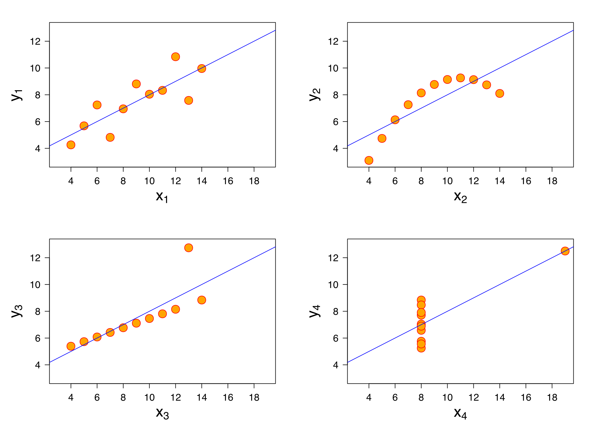
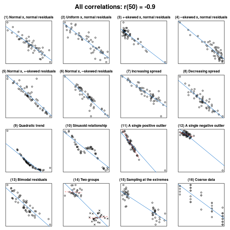
Jan Vanhove What data patterns can lie behind a correlation coefficient?.
7.1 Linear regressions
The most basic form is a simple linear regression that can be performed directly in R using the function lm(). In this case, we have to two vectors with paired responses where a measurement of one predictor usually represented as x is corresponded with one dependent response represented as y.
For this example, we will use the R-package MASS and its dataset mammals that contains brain and body weights for 62 species of land mammals.
## we can install MASS and load the dataset mammals for this example
install.packages("MASS")
library(MASS)
?mammals
# assign mammals dataset to an object
mammals_raw <- mammals
head(mammals_raw)
#                   body brain
#Arctic fox        3.385  44.5
#Owl monkey        0.480  15.5
#Mountain beaver   1.350   8.1
#Cow             465.000 423.0
#Grey wolf        36.330 119.5
#Goat             27.660 115.0
We can explore the relationship of bodyas predictor of brain by plotting their one-to-one relationship. Notice the formula brain ~ body inside the regression function lm() that correspond brain (y-axis) and body (x-axis).
plot(x = mammals_raw$body, y = mammals_raw$brain)
mtext(side=3, line=0.5, adj=0, "raw data from mammal -- body vs brain")
abline(lm(brain ~ body, data = mammals_raw), col = "blue")

# let's save this model to an object
raw_brain_body <- lm(brain ~ body, data = mammals_raw)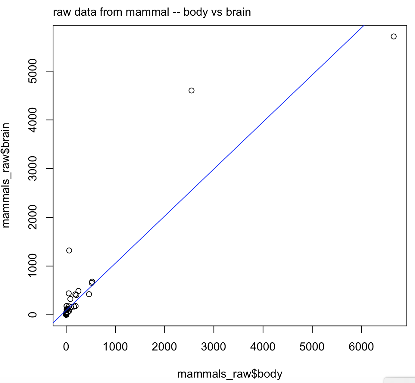
What do you see in this plot? It suggests that brain and body might not have a quite linear relationship. The reason is a well-known exponential relationship between body and brain size.
We need to transform the data, which includes taking the log10 of both variables. For this transformation, we can use the function modify() of the package purrr
# we have already downloaded this function before
library(purrr)
mammals_log <- modify(mammals_raw,log10)
head(mammals_log)
#                     body    brain
#Arctic fox       0.5295587 1.648360
#Owl monkey      -0.3187588 1.190332
#Mountain beaver  0.1303338 0.908485
#Cow              2.6674530 2.626340
#Grey wolf        1.5602654 2.077368
#Goat             1.4418522 2.060698

# now we can plot this transformed data
plot(x = mammals_log$body, y = mammals_log$brain)
mtext(side=3, line=0.5, adj=0, "Log10 data from mammal -- body vs brain")
abline(lm(brain ~ body, data = mammals_log), col = "blue")

# let's save this model to an object
log_brain_body <- lm(brain ~ body, data = mammals_log)
# class of this regression object is "lm".
class(log_brain_body)
#[1] "lm"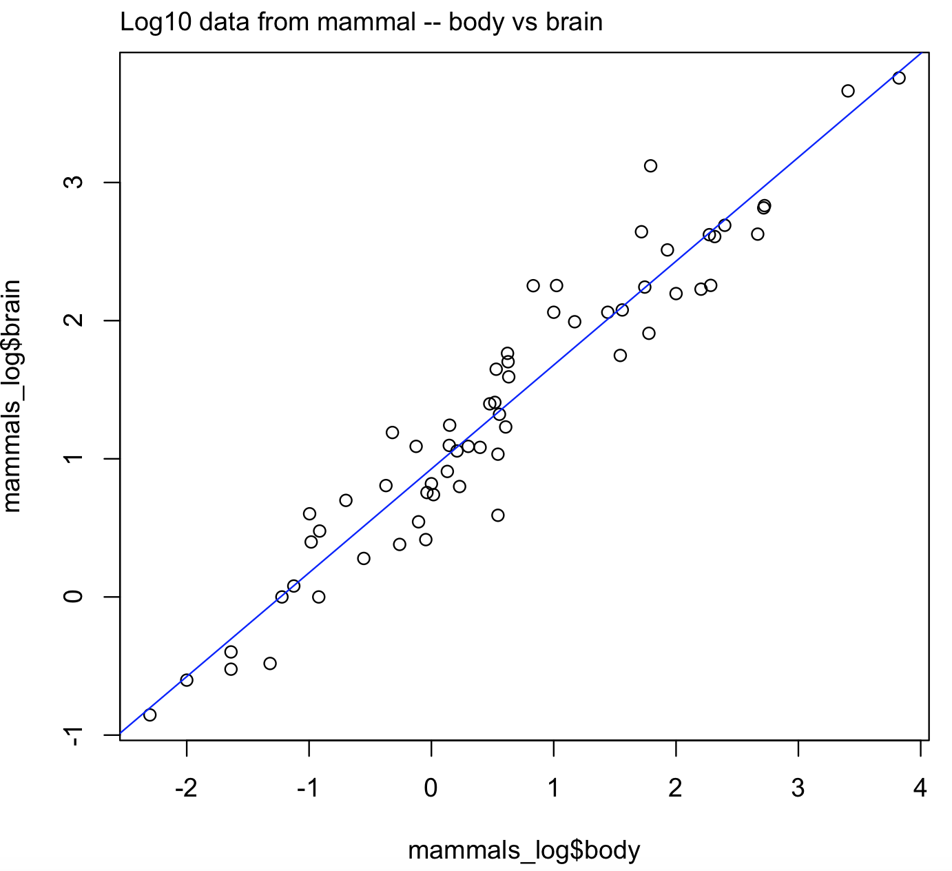
This is a better plot and it is easier to visualize the linear trend in the log10 transformed data for body and brain sizes.
We can summarize the results of these simple linear regressions with the function summary().
First, we need to understand significance values and symbols (i.e., the asterisks *) next to sections of the output
| Symbol | p-value range | Interpretation |
|---|---|---|
| *** | less than 0.001 | strongly significant and very likely to reject null (e.g., coefficient different than 0) |
| ** | 0.001 < p-value < 0.01 | significant and most likely to reject null (e.g., coefficient different than 0) |
| * | 0.05 < p-value < 0.1 | barely significant and likely to reject null (e.g., coefficient different than 0) |
| . | p-value > 0.05 | likely not significant and might not reject null (e.g., coefficient different than 0) |
| no- asterisks | p-value > 0.05 | does not reject null (e.g., coefficient is not different than 0) |
## summary for the untransformed data
summary(raw_brain_body)
#Call:
#lm(formula = brain ~ body, data = mammals_raw)
#
#Residuals:
#    Min      1Q  Median      3Q     Max
#-810.07  -88.52  -79.64  -13.02 2050.33
#
#Coefficients:
#            Estimate Std. Error t value Pr(>|t|)
#(Intercept) 91.00440   43.55258    2.09   0.0409 *
#body         0.96650    0.04766   20.28   <2e-16 ***
#---
#Signif. codes:  0 ‘***’ 0.001 ‘**’ 0.01 ‘*’ 0.05 ‘.’ 0.1 ‘ ’ 1
#
#Residual standard error: 334.7 on 60 degrees of freedom
#Multiple R-squared:  0.8727,   Adjusted R-squared:  0.8705
#F-statistic: 411.2 on 1 and 60 DF,  p-value: < 2.2e-16

## summary for the log10 transformed data
Some of the highlights of the raw_brain_body output are as follows:
| Coefficient name | Coefficient value | Statistic name | Statistic value | p-value | Interpretation |
|---|---|---|---|---|---|
| F | 411.2 | < 2.2e-16 *** | the model is strongly significant | ||
| Intercept | 91.00440 | t-value | 2.09 | 0.0409 * | Intercept coefficient is barely significant |
| Body | 0.96650 | t-value | 20.28 | < 2.2e-16 *** | Body coefficient is strongly significant |
| R-squared | 0.8727 | the value is close to 1.0 and model is useful |
summary(log_brain_body)
#Call:
#lm(formula = brain ~ body, data = mammals_log)
#
#Residuals:
#     Min       1Q   Median       3Q      Max
#-0.74503 -0.21380 -0.02676  0.18934  0.84613
#
#Coefficients:
#            Estimate Std. Error t value Pr(>|t|)
#(Intercept)  0.92713    0.04171   22.23   <2e-16 ***
#body         0.75169    0.02846   26.41   <2e-16 ***
#---
#Signif. codes:  0 ‘***’ 0.001 ‘**’ 0.01 ‘*’ 0.05 ‘.’ 0.1 ‘ ’ 1
#
#Residual standard error: 0.3015 on 60 degrees of freedom
#Multiple R-squared:  0.9208,   Adjusted R-squared:  0.9195
#F-statistic: 697.4 on 1 and 60 DF,  p-value: < 2.2e-16
Some of the highlights of the log_brain_body output can be as follows.
| Coefficient name | Coefficient value | Statistic name | Statistic value | p-value | Interpretation |
|---|---|---|---|---|---|
| F | 697.4 | < 2.2e-16 *** | the model is strongly significant | ||
| Intercept | 0.92713 | t-value | 22.23 | < 2.2e-16 *** | Intercept coefficient is strongly significant |
| Body | 0.75169 | t-value | 26.41 | < 2.2e-16 *** | body coefficient is strongly significant |
| R-squared | 0.9208 | the value is close to 1.0 and model is useful |
We can conclude that both models are significant and useful, but the model based on a log10 transformed data seems to have a better fit for a linear regression model (e.g., see intercept row).
7.2 Anatomy of a linear regression
In most cases, you will import your dataset directly into R rather than getting it from a default dataset. you should follow section 2.6 instructions for details.
Here, we will do that with an example in our class GitHub repository
called MASS_crabs_dataset.xlsx. You can download this file to your working directory.
## we get the crabs from MASS
library(MASS)
?crabs

## load the crab dataset
crab_dataset <- crabs

head(crab_dataset)
#  sp sex index   FL  RW   CL   CW  BD
#1  B   M     1  8.1 6.7 16.1 19.0 7.0
#2  B   M     2  8.8 7.7 18.1 20.8 7.4
#3  B   M     3  9.2 7.8 19.0 22.4 7.7
#4  B   M     4  9.6 7.9 20.1 23.1 8.2
#5  B   M     5  9.8 8.0 20.3 23.0 8.2
#6  B   M     6 10.8 9.0 23.0 26.5 9.8

## explore your data
str(crab_dataset)
#'data.frame':   200 obs. of  8 variables:
# $ sp   : chr  "B" "B" "B" "B" ...
# $ sex  : chr  "M" "M" "M" "M" ...
# $ index: num  1 2 3 4 5 6 7 8 9 10 ...
# $ FL   : num  8.1 8.8 9.2 9.6 9.8 10.8 11.1 11.6 11.8 11.8 ...
# $ RW   : num  6.7 7.7 7.8 7.9 8 9 9.9 9.1 9.6 10.5 ...
# $ CL   : num  16.1 18.1 19 20.1 20.3 23 23.8 24.5 24.2 25.2 ...
# $ CW   : num  19 20.8 22.4 23.1 23 26.5 27.1 28.4 27.8 29.3 ...
# $ BD   : num  7 7.4 7.7 8.2 8.2 9.8 9.8 10.4 9.7 10.3 ...
For this example, we have loaded the same dataset called crab_dataset that has morphological measurements on Leptograpsus crabs that is from a collection of datasets in the R-package MASS.
The variables that included are sp for a discrete variable for species named “B” or “O” (blue or orange),
sex (discrete for M-male and F-female), index as an index from 1 to 50 within each of the four groups of this dataset, FL is frontal lobe size (mm),
RW is rear width size (mm), CL is carapace length size (mm), CW is carapace width size (mm), and BD is
body depth size (mm).
We can perform a simple linear regression with BD as a dependent variable and FL as a predictor.
## This is the code for this regression
crab_simple_lm <- lm(formula = BD ~ FL, data = crab_dataset)
In the code above, we have the following components. The lm() is the function for Fitting Linear Models.
The arguments for this function include formula with a dependent variable (i.e., this is the y in most statistics courses)
named BD or the carb population measurement of body depth size (mm); a ~ (i.e., this is the = in most statistics courses);
an independent or predictor variable (i.e., this is the x in most statistics courses)
named FL or the carb population measurement of frontal lobe size (mm). Finally, data is the argument that has the name of the object that contains the data to be used in the
regression (i.e., crab_dataset).
## We can get the summary of this regression to determine if usefulness
summary(crab_simple_lm)

#Call:
#lm(formula = BD ~ FL, data = crab_dataset)
#
#Residuals:
#    Min      1Q  Median      3Q     Max
#-1.9500 -0.3035  0.0302  0.3563  1.1692
#
#Coefficients:
#            Estimate Std. Error t value Pr(>|t|)
#(Intercept) -1.04904    0.17437  -6.016 8.49e-09 ***
#FL           0.96769    0.01092  88.618  < 2e-16 ***
#---
#Signif. codes:  0 ‘***’ 0.001 ‘**’ 0.01 ‘*’ 0.05 ‘.’ 0.1 ‘ ’ 1
#
#Residual standard error: 0.5384 on 198 degrees of freedom
#Multiple R-squared:  0.9754,    Adjusted R-squared:  0.9753
#F-statistic:  7853 on 1 and 198 DF,  p-value: < 2.2e-16
Based on these statistics, this regression is significant (F-statistic with a p-value <0.0001), the model seems to be useful (R-squared is very close to 1 as 0.9753), and the FL regression coefficients was positive (i.e., 0.96769, and indicates that as BD increases, FL also increases) and significant (t-statistic with a p-value <0.0001). We can conclude that body depth (BD) increases can be predicted with increases of frontal lobe (FL) size in the population of crabs studied.
7.3 Multiple linear regressions
We can expand our regression models to more than one predictor (i.e., multiple linear regression) that can be performed again using the same lm() function. In this case, we have multiple (several) predictors for our dependent variable.
For this example, we will continue to use the crabs dataset that has morphological measurements on Leptograpsus crabs from the R-package MASS.
## we have already downloaded MASS and we assign the crabs dataset to an object
library(MASS)
crab_dataset <- crabs
head(crab_dataset)
#  sp sex index   FL  RW   CL   CW  BD
#1  B   M     1  8.1 6.7 16.1 19.0 7.0
#2  B   M     2  8.8 7.7 18.1 20.8 7.4
#3  B   M     3  9.2 7.8 19.0 22.4 7.7
#4  B   M     4  9.6 7.9 20.1 23.1 8.2
#5  B   M     5  9.8 8.0 20.3 23.0 8.2
#6  B   M     6 10.8 9.0 23.0 26.5 9.8

## we will use BD as dependent and FL, RW, CL and CW as predictors.
crab_multiple_lm <- lm(formula = BD ~ FL+RW+CL+CW, data = crab_dataset)
class(crab_multiple_lm)
#[1] "lm"
summary(crab_multiple_lm)
#Call:
#lm(formula = BD ~ FL + RW + CL + CW, data = crab_dataset)
#
#Residuals:
#    Min      1Q  Median      3Q     Max
#-1.3518 -0.2291  0.0112  0.2664  1.0965
#
#Coefficients:
#            Estimate Std. Error t value Pr(>|t|)
#(Intercept) -0.97616    0.15296  -6.382 1.25e-09 ***
#FL           0.42022    0.05585   7.524 1.91e-12 ***
#RW           0.03768    0.03209   1.174    0.242
#CL           0.59511    0.06825   8.720 1.22e-15 ***
#CW          -0.30560    0.04935  -6.193 3.43e-09 ***
#---
#Signif. codes:  0 ‘***’ 0.001 ‘**’ 0.01 ‘*’ 0.05 ‘.’ 0.1 ‘ ’ 1
#
#Residual standard error: 0.4208 on 195 degrees of freedom
#Multiple R-squared:  0.9852,   Adjusted R-squared:  0.9849
#F-statistic:  3247 on 4 and 195 DF,  p-value: < 2.2e-16
Based on these statistics, the multiple regression is significant (F-statistic with a p-value <0.0001). Likewise, the model seems to be useful in predicting BD values (Multiple R-squared is very close to 1) and all coefficients with the exception for CL (carapace length) were significant.
7.4 Diagnostic plots for regressions
We can perform some diagnostic plots to checks for heteroscedasticity, normality, and influential observerations.
# diagnostic plots
layout(matrix(c(1,2,3,4),2,2))
plot(crab_multiple_lm)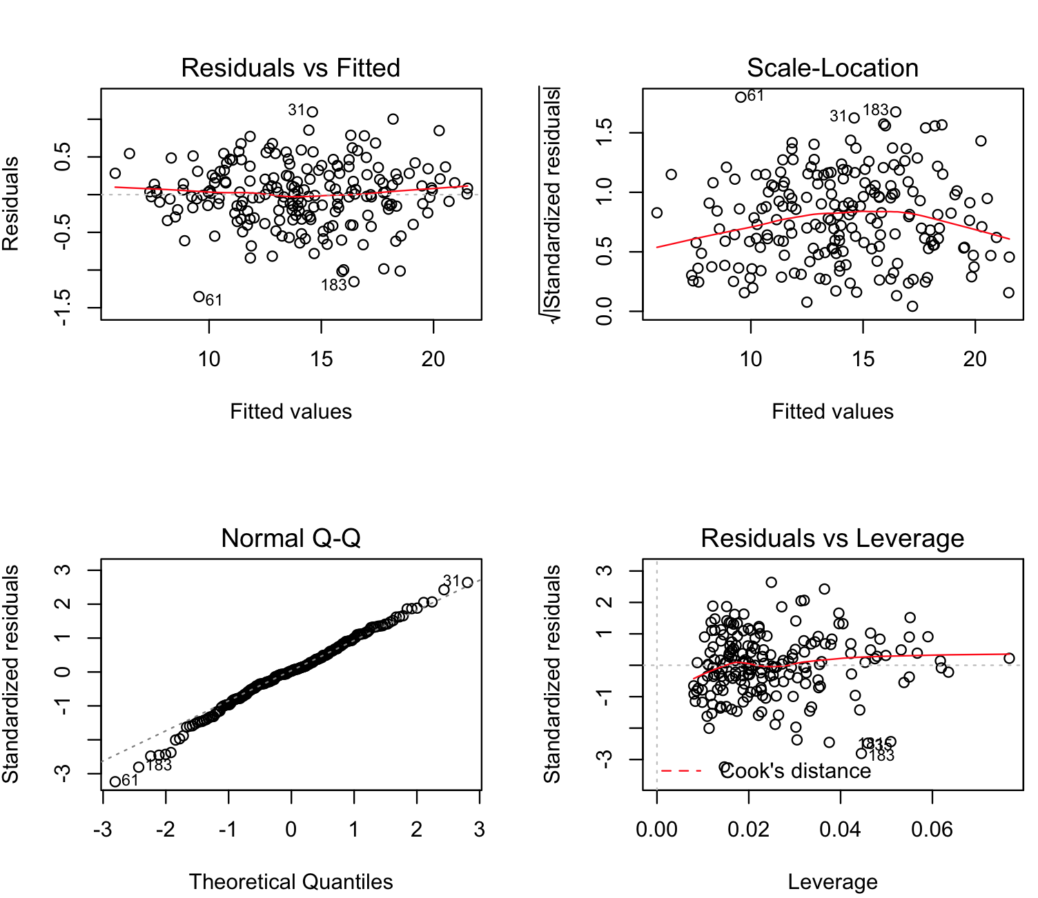
To understand these plots, we need to look for indications that data might not follow normality or has bias. These include:
(a) the Residual vs Fitted should have a random distribution without any pattern (our plot shows that).
(b) the Normal Q-Q show fall into oblique dashed line that supports relative multivariate normality (i.e., our multiple linear method is valid).
(c) the plots Scale-Location and Residuals vs Leverage should fall close to the center (i.e., these plots are more or less OK).
7.5 Regression influential measurements
You can also get a list of influential measurements using functions influence.measures() and influence(). These measurements might be outliers or errors in data input (i.e., miss typing, incorrect instrument calibration, contamination, etc.)
## Notice values with an asterisk (*)
influence_values <- influence.measures(crab_multiple_lm)
influence_values
#Influence measures of
#    lm(formula = BD ~ FL + RW + CL + CW, data = crab_dataset) :
#
#       dfb.1_    dfb.FL    dfb.RW    dfb.CL    dfb.CW     dffit cov.r   cook.d     hat inf
#1    0.230383  1.06e-01 -1.27e-01 -1.15e-01  9.97e-02  0.272172 1.022 1.48e-02 0.04052
#2   -0.009954 -4.12e-05  1.55e-03 -6.81e-05  5.21e-04 -0.010550 1.053 2.24e-05 0.02556
#3    0.018286  6.27e-03 -9.58e-03 -9.30e-03  9.08e-03  0.022461 1.056 1.01e-04 0.02866
#...
#46   0.076014 -8.84e-02  2.99e-01  1.25e-01 -1.87e-01 -0.426499 0.914 3.55e-02 0.03051   *
#47   0.037663 -1.85e-02  3.83e-02  4.76e-02 -6.15e-02 -0.088701 1.057 1.58e-03 0.03509
#48  -0.027395  8.70e-03 -7.23e-02 -3.70e-02  6.03e-02  0.115458 1.077 2.68e-03 0.05319   *
#49  -0.017943  1.88e-02 -4.78e-02 -3.53e-02  4.67e-02  0.071147 1.077 1.02e-03 0.04985   *
#50  -0.023874  7.47e-05 -3.10e-02 -2.11e-02  3.51e-02  0.063645 1.110 8.14e-04 0.07675   *
#51   0.127156  8.62e-03 -2.53e-02 -8.99e-03  2.53e-03  0.133549 1.052 3.58e-03 0.03666
#32  -0.020620 -6.29e-02 -1.96e-02 -3.45e-03  4.20e-02  0.145671 1.028 4.25e-03 0.02396
#...

## now we can get the identity of these values organized in a vector by focusing in column 'hat'
influence_df <- influence(crab_multiple_lm)
head(influence_df)
# we can the 10 most influential value
order(influence_df$hat, decreasing = TRUE)[1:10]
#[1]  50 145 199 195  98 200  99 144 186  97
7.6 Regression coefficients and their 95%CI
We can further explore our simple and multiple regression examples by calling different regression statistics. We have two regression objects log_brain_body and crab_multiple_lm.
Get the model coefficients using the function coefficients() or coef().
coefficients(log_brain_body)
#(Intercept)        body
#  0.9271269   0.7516859
coef(crab_multiple_lm)
#(Intercept)          FL          RW          CL          CW
#-0.97615668  0.42022057  0.03768281  0.59511478 -0.30559587
Get the model confidence intervals for regression coefficients (i.e., range that contains the estimate regression coefficients) using the function confint().
confint(log_brain_body)
#                2.5 %    97.5 %
#(Intercept) 0.8436923 1.0105616
#body        0.6947503 0.8086215
confint(crab_multiple_lm)
#                  2.5 %     97.5 %
#(Intercept) -1.27783361 -0.6744798
#FL           0.31007030  0.5303708
#RW          -0.02560597  0.1009716
#CL           0.46051803  0.7297115
#CW          -0.40291710 -0.2082746
Notice the confidence interval for RW is (-0.02560597, 0.1009716) and this range contains 0.0 (i.e., zero). This is consistent with the summary(crab_multiple_lm) where RW was not significant.
ANOVA table, we will explore this later in this session. We use the function anova().
anova(log_brain_body)
#Analysis of Variance Table
#
#Response: brain
#          Df Sum Sq Mean Sq F value    Pr(>F)
#body       1 63.409  63.409  697.42 < 2.2e-16 ***
#Residuals 60  5.455   0.091
#---
#Signif. codes:  0 ‘***’ 0.001 ‘**’ 0.01 ‘*’ 0.05 ‘.’ 0.1 ‘ ’ 1
anova(crab_multiple_lm)
#Analysis of Variance Table
#
#Response: BD
#           Df  Sum Sq Mean Sq    F value    Pr(>F)
#FL          1 2276.68 2276.68 12858.0018 < 2.2e-16 ***
#RW          1    0.57    0.57     3.1984   0.07526 .
#CL          1   15.52   15.52    87.6332 < 2.2e-16 ***
#CW          1    6.79    6.79    38.3516  3.43e-09 ***
#Residuals 195   34.53    0.18
#---
#Signif. codes:  0 ‘***’ 0.001 ‘**’ 0.01 ‘*’ 0.05 ‘.’ 0.1 ‘ ’ 1
7.7 Selecting predictors
We can further improve our regression by selecting the best predictors and removing those that do not contribute to the regression. The function step() can help you to determine what predictors to keep .
We will illustrate this using our model crab_multiple_lm.
## we will assign this as our full model
full_model <- crab_multiple_lm
full_model
#Call:
#lm(formula = BD ~ FL + RW + CL + CW, data = crab_dataset)
#
#Coefficients:
#(Intercept)           FL           RW           CL           CW
#  -0.97616      0.42022      0.03768      0.59511     -0.30560
We can do this using backward or both approaches (they usually reach the same conclusion).
reduced_model <- step(full_model, direction = "backward")
#Start:  AIC=-341.31
#BD ~ FL + RW + CL + CW
#
#       Df Sum of Sq    RSS     AIC
#- RW    1    0.2442 34.772 -341.90
#<none>              34.527 -341.31
#- CW    1    6.7907 41.318 -307.40
#- FL    1   10.0234 44.551 -292.34
#- CL    1   13.4637 47.991 -277.46

#Step:  AIC=-341.9
#BD ~ FL + CL + CW
#
#       Df Sum of Sq    RSS     AIC
#<none>              34.772 -341.90
#- CW    1    7.5018 42.273 -304.83
#- CL    1   15.2099 49.981 -271.33
#- FL    1   17.0716 51.843 -264.02
reduced_model
#
#Call:
#lm(formula = BD ~ FL + CL + CW, data = crab_dataset)
#
#Coefficients:
#(Intercept)           FL           CL           CW
We can notice that the predictor RW has been dropped from the reduced model and we can get some statistics on this improved model.
summary(reduced_model)
#Call:
#lm(formula = BD ~ FL + CL + CW, data = crab_dataset)
#
#Residuals:
#     Min       1Q   Median       3Q      Max
#-1.34264 -0.23109  0.00893  0.26523  1.05895
#
#Coefficients:
#            Estimate Std. Error t value Pr(>|t|)
#(Intercept) -0.92444    0.14663  -6.305 1.87e-09 ***
#FL           0.45656    0.04654   9.810  < 2e-16 ***
#CL           0.55718    0.06018   9.259  < 2e-16 ***
#CW          -0.27594    0.04243  -6.503 6.41e-10 ***
#---
#Signif. codes:  0 ‘***’ 0.001 ‘**’ 0.01 ‘*’ 0.05 ‘.’ 0.1 ‘ ’ 1
#
#Residual standard error: 0.4212 on 196 degrees of freedom
#Multiple R-squared:  0.9851,   Adjusted R-squared:  0.9849
#F-statistic:  4320 on 3 and 196 DF,  p-value: < 2.2e-16
7.8 Regression predictions
One of the most important uses of regressions is predictions of the dependent variable. For example, given a set of measurements on your predictors, can you predict an outcome. This can be done using the function predict().
As an example, we will predict brain size of some mammals that are not in the mammals_raw dataset.
## recall the regression and the predictor name for the model: log_brain_body
log_brain_body
#Call:
#lm(formula = brain ~ body, data = mammals_log)
#
#Coefficients:
#(Intercept)         body
#     0.9271       0.7517
We cab revise species in mammals_raw.
head(mammals_raw)
#                   body brain
#Arctic fox        3.385  44.5
#Owl monkey        0.480  15.5
#Mountain beaver   1.350   8.1
#Cow             465.000 423.0
#Grey wolf        36.330 119.5
#Goat             27.660 115.0
rownames(mammals_raw)
#[1] "Arctic fox"                "Owl monkey"                "Mountain beaver"           "Cow"
# [5] "Grey wolf"                 "Goat"                      "Roe deer"                  "Guinea pig"
# [9] "Verbet"                    "Chinchilla"                "Ground squirrel"           "Arctic ground squirrel"
#[13] "African giant pouched rat" "Lesser short-tailed shrew" "Star-nosed mole"           "Nine-banded armadillo"
#[17] "Tree hyrax"                "N.A. opossum"              "Asian elephant"            "Big brown bat"
#[21] "Donkey"                    "Horse"                     "European hedgehog"         "Patas monkey"
#[25] "Cat"                       "Galago"                    "Genet"                     "Giraffe"
#[29] "Gorilla"                   "Grey seal"                 "Rock hyrax-a"              "Human"
#[33] "African elephant"          "Water opossum"             "Rhesus monkey"             "Kangaroo"
#[37] "Yellow-bellied marmot"     "Golden hamster"            "Mouse"                     "Little brown bat"
#[41] "Slow loris"                "Okapi"                     "Rabbit"                    "Sheep"
#[45] "Jaguar"                    "Chimpanzee"                "Baboon"                    "Desert hedgehog"
#[49] "Giant armadillo"           "Rock hyrax-b"              "Raccoon"                   "Rat"
#[53] "E. American mole"          "Mole rat"                  "Musk shrew"                "Pig"
#[57] "Echidna"                   "Brazilian tapir"           "Tenrec"                    "Phalanger"
#[61] "Tree shrew"                "Red fox"
We will add three more mammals body weight in kg and estimate their brain weight in g by create a new data frame with the new body sizes.
new_body <- data.frame(body = c(272, 495, 160, 3.13), stringsAsFactors = FALSE)
rownames(new_body) <- c("grizzly_bear", "bactrian_camel", "llama", "capuchin_monkey")
new_body
#                  body
#grizzly_bear    272.00
#bactrian_camel  495.00
#llama           160.00
#capuchin_monkey   3.13
Remember that the model is for log10 transformed data, so we need to transform accordingly.
library(purrr)
new_body_log <- purrr::modify(new_body,log10)
rownames(new_body_log) <- rownames(new_body)
new_body_log
#                     body
#grizzly_bear    2.4345689
#bactrian_camel  2.6946052
#llama           2.2041200
#capuchin_monkey 0.4955443
We can estimate their brain weight in g of these mammals using the function predict().
new_brain_log <- predict(log_brain_body, new_body_log)
new_brain_log
#   grizzly_bear  bactrian_camel           llama capuchin_monkey
#      2.757158        2.952624        2.583933        1.299621
We can transform this log10 weight brains back by exponentiation with base 10.
new_brain <- 10^new_brain_log
new_brain
#   grizzly_bear  bactrian_camel           llama capuchin_monkey
#       571.6868        896.6517        383.6480         19.9352
7.9 Logistic regressions
We can use a logistic regression when our dependent variable is binary (i.e., 1 or 0; yes or no; A or B; male or female) from a set of continuous predictor variables that determine such outcome. We can implement such regressions using the function glm() for a generalized linear model (GLM).
We will dataset catsthat has anatomical data from domestic cats including sex and two continuous variables (body and heart weight). This dataset is part of the R-package MASS.
## load MASS package and ‘cats’ dataset
library(MASS)
?cats
cats_data <- cats
# check structure
str(cats_data)
#'data.frame':  144 obs. of  3 variables:
# $ Sex: Factor w/ 2 levels "F","M": 1 1 1 1 1 1 1 1 1 1 ...
# $ Bwt: num  2 2 2 2.1 2.1 2.1 2.1 2.1 2.1 2.1 ...
# $ Hwt: num  7 7.4 9.5 7.2 7.3 7.6 8.1 8.2 8.3 8.5 ...
We can now run the model with the formula with Sex as a binary dependent and the two continuous as predictors: Body weight Bwt and heart weight Hwt. Notice the argument for type or family of distribution family = binomial() for these logistic regressions.
cats_data_logistic_fit <- glm(Sex ~ Bwt + Hwt, data = cats_data, family = binomial())
summary(cats_data_logistic_fit)
#Call:
#glm(formula = Sex ~ Bwt + Hwt, family = binomial(), data = cats_data)
#
#Deviance Residuals:
#    Min       1Q   Median       3Q      Max
#-2.1727  -0.7815   0.3141   0.7476   1.8189
#
#Coefficients:
#            Estimate Std. Error z value Pr(>|z|)
#(Intercept) -8.69896    1.69982  -5.118 3.09e-07 ***
#Bwt          3.55391    0.88208   4.029 5.60e-05 ***
#Hwt          0.02295    0.16146   0.142    0.887
#---
#Signif. codes:  0 ‘***’ 0.001 ‘**’ 0.01 ‘*’ 0.05 ‘.’ 0.1 ‘ ’ 1
#
#(Dispersion parameter for binomial family taken to be 1)
#
#    Null deviance: 181.90  on 143  degrees of freedom
#Residual deviance: 132.24  on 141  degrees of freedom
#AIC: 138.24
#
#Number of Fisher Scoring iterations: 5
For the summary, we can that the intercept and body weight (Bwt) are strongly significant, while heart weight (Hwt) is not. This suggest that the sex of the cat has a strong association of the weight of the cat, while not its heart weight. For body weight, its regression coefficient is positive (3.55391) and it suggests that heavier cats are most likely to be males while controlling for their heart weight.
Now, we can plot this logistic regression:
cats_data_newdata <- expand.grid(Bwt = pretty(cats_data$Bwt, 20), Hwt = pretty(cats_data$Hwt, 5))
cats_data_newdata$Sex <- predict(cats_data_logistic_fit, newdata = cats_data_newdata, type = "response")
## we require library ggplot2
library(ggplot2)
ggplot(cats_data_newdata, aes(x = Bwt, y = Sex)) + geom_line() + facet_wrap(~Hwt)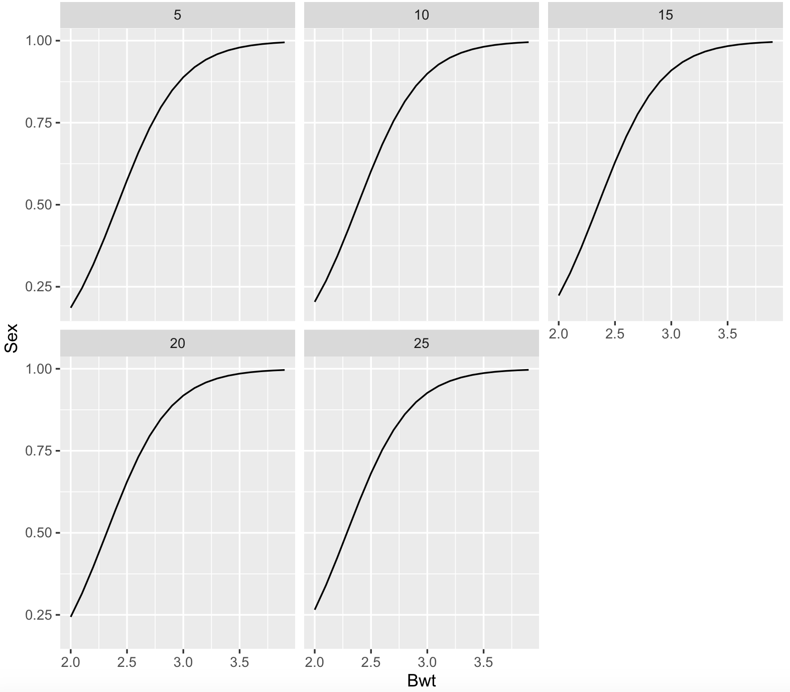
7.10 Logistic regressions requirements
It is important that the dependent variable is a binary variable such as a factor with two levels or in the form of 0 and 1, otherwise the logistic regression function might not accept your data input. We will do an example with the Cars93 dataset form R-package MASS.
library(MASS)
my_cars <- Cars93
?Cars93
str(my_cars)
#'data.frame':  93 obs. of  27 variables:
# $ Manufacturer      : Factor w/ 32 levels "Acura","Audi",..: 1 1 2 2 3 4 4 4 4 5 ...
# $ Model             : Factor w/ 93 levels "100","190E","240",..: 49 56 9 1 6 24 54 74 73 35 ...
# $ Type              : Factor w/ 6 levels "Compact","Large",..: 4 3 1 3 3 3 2 2 3 2 ...
# $ Min.Price         : num  12.9 29.2 25.9 30.8 23.7 14.2 19.9 22.6 26.3 33 ...
# $ Price             : num  15.9 33.9 29.1 37.7 30 15.7 20.8 23.7 26.3 34.7 ...
# $ Max.Price         : num  18.8 38.7 32.3 44.6 36.2 17.3 21.7 24.9 26.3 36.3 ...
# $ MPG.city          : int  25 18 20 19 22 22 19 16 19 16 ...
# $ MPG.highway       : int  31 25 26 26 30 31 28 25 27 25 ...
# $ AirBags           : Factor w/ 3 levels "Driver & Passenger",..: 3 1 2 1 2 2 2 2 2 2 ...
# $ DriveTrain        : Factor w/ 3 levels "4WD","Front",..: 2 2 2 2 3 2 2 3 2 2 ...
# $ Cylinders         : Factor w/ 6 levels "3","4","5","6",..: 2 4 4 4 2 2 4 4 4 5 ...
# $ EngineSize        : num  1.8 3.2 2.8 2.8 3.5 2.2 3.8 5.7 3.8 4.9 ...
# $ Horsepower        : int  140 200 172 172 208 110 170 180 170 200 ...
# $ RPM               : int  6300 5500 5500 5500 5700 5200 4800 4000 4800 4100 ...
# $ Rev.per.mile      : int  2890 2335 2280 2535 2545 2565 1570 1320 1690 1510 ...
# $ Man.trans.avail   : Factor w/ 2 levels "No","Yes": 2 2 2 2 2 1 1 1 1 1 ...
# $ Fuel.tank.capacity: num  13.2 18 16.9 21.1 21.1 16.4 18 23 18.8 18 ...
# $ Passengers        : int  5 5 5 6 4 6 6 6 5 6 ...
# $ Length            : int  177 195 180 193 186 189 200 216 198 206 ...
# $ Wheelbase         : int  102 115 102 106 109 105 111 116 108 114 ...
# $ Width             : int  68 71 67 70 69 69 74 78 73 73 ...
# $ Turn.circle       : int  37 38 37 37 39 41 42 45 41 43 ...
# $ Rear.seat.room    : num  26.5 30 28 31 27 28 30.5 30.5 26.5 35 ...
# $ Luggage.room      : int  11 15 14 17 13 16 17 21 14 18 ...
# $ Weight            : int  2705 3560 3375 3405 3640 2880 3470 4105 3495 3620 ...
# $ Origin            : Factor w/ 2 levels "USA","non-USA": 2 2 2 2 2 1 1 1 1 1 ...
# $ Make              : Factor w/ 93 levels "Acura Integra",..: 1 2 4 3 5 6 7 9 8 10 ...

## we will try to determine if Origin is predicted by Price.

price_logistic_fit <- glm(Origin ~ Price, data = my_cars, family = binomial())
summary(price_logistic_fit)
#
# Call:
# glm(formula = Origin ~ Price, family = binomial(), data = my_cars)
#
# Deviance Residuals:
#    Min      1Q  Median      3Q     Max
# -1.340  -1.122  -1.058   1.209   1.311
#
# Coefficients:
#             Estimate Std. Error z value Pr(>|z|)
# (Intercept) -0.47995    0.47851  -1.003    0.316
# Price        0.02131    0.02217   0.961    0.336
#
# (Dispersion parameter for binomial family taken to be 1)
#
#     Null deviance: 128.83  on 92  degrees of freedom
# Residual deviance: 127.88  on 91  degrees of freedom
# AIC: 131.88
#
# Number of Fisher Scoring iterations: 4
In this case, price does not predict the car Origin (i.e., if car is made in USA and non-USA).
However, we can repeat this analysis but by assuming that Origin variable is character and not a factor.
my_car_origin_price <- subset(Cars93, select = c(Origin, Price))
str(my_car_origin_price)
# 'data.frame': 93 obs. of  2 variables:
# $ Origin: Factor w/ 2 levels "USA","non-USA": 2 2 2 2 2 1 1 1 1 1 ...
# $ Price : num  15.9 33.9 29.1 37.7 30 15.7 20.8 23.7 26.3 34.7 ...

## now, we transform Origin into a character variable
my_car_origin_price$Origin <- as.character(my_car_origin_price$Origin)
str(my_car_origin_price)
# 'data.frame':   93 obs. of  2 variables:
# $ Origin: chr  "non-USA" "non-USA" "non-USA" "non-USA" ...
# $ Price : num  15.9 33.9 29.1 37.7 30 15.7 20.8 23.7 26.3 34.7 ...

## we repeat the analysis, and we get an error
price_logistic_fit <- glm(Origin ~ Price, data = my_car_origin_price, family = binomial())
# Error in eval(family$initialize) : y values must be 0 <= y <= 1

## we get this error and we need to make it binary (0 and 1) or a factor
## 0 will be non-USA and 1 will be USA
my_car_origin_price$Origin <- ifelse(my_car_origin_price$Origin == "USA", 1,0)
head(my_car_origin_price)
#  Origin Price
#1      0  15.9
#2      0  33.9
#3      0  29.1
#4      0  37.7
#5      0  30.0
#6      1  15.7

## we repeat the analysis, it works now, and we get the same result
price_logistic_fit <- glm(Origin ~ Price, data = my_car_origin_price, family = binomial())
summary(price_logistic_fit)
#
# Call:
# glm(formula = Origin ~ Price, family = binomial(), data = my_cars)
#
# Deviance Residuals:
#    Min      1Q  Median      3Q     Max
# -1.340  -1.122  -1.058   1.209   1.311
#
# Coefficients:
#             Estimate Std. Error z value Pr(>|z|)
# (Intercept) -0.47995    0.47851  -1.003    0.316
# Price        0.02131    0.02217   0.961    0.336
#
# (Dispersion parameter for binomial family taken to be 1)
#
#     Null deviance: 128.83  on 92  degrees of freedom
# Residual deviance: 127.88  on 91  degrees of freedom
# AIC: 131.88
#
# Number of Fisher Scoring iterations: 4
In other instances, you might want to binarize a continuous variable so you can apply a logistic regression.
We can try by binirizing the variable MPG.city for low_milage or 1 if less 20 mpg and all other as high_milage or 0 (i.e., their mpg > 20).
Our predictor will be Price again.
my_car_mpg_price <- subset(Cars93, select = c(MPG.city, Price))
str(my_car_mpg_price)
#'data.frame':   93 obs. of  2 variables:
# $ MPG.city: int  25 18 20 19 22 22 19 16 19 16 ...
# $ Price   : num  15.9 33.9 29.1 37.7 30 15.7 20.8 23.7 26.3 34.7 ...

## we can binarize MPG.city as 0 and 1
my_car_mpg_price$binary_mpg <- ifelse(my_car_mpg_price$MPG.city <=20,1,0)
str(my_car_mpg_price)
#'data.frame':  93 obs. of  3 variables:
# $ MPG.city  : int  25 18 20 19 22 22 19 16 19 16 ...
# $ Price     : num  15.9 33.9 29.1 37.7 30 15.7 20.8 23.7 26.3 34.7 ...
# $ binary_mpg: num  0 1 1 1 0 0 1 1 1 1 ...

## we will try to determine if binary_mpg is predicted by Price.
mpg_logistic_fit <- glm(binary_mpg ~ Price, data = my_car_mpg_price, family = binomial())
summary(mpg_logistic_fit)
#
# Call:
# glm(formula = binary_mpg ~ Price, family = binomial(), data = my_car_mpg_price)
#
# Deviance Residuals:
#    Min       1Q   Median       3Q      Max
# -2.8353  -0.5372  -0.2289   0.3939   1.9267
#
# Coefficients:
#             Estimate Std. Error z value Pr(>|z|)
# (Intercept) -6.59673    1.40187  -4.706 2.53e-06 ***
# Price        0.35327    0.07742   4.563 5.04e-06 ***
# ---
# Signif. codes:  0 ‘***’ 0.001 ‘**’ 0.01 ‘*’ 0.05 ‘.’ 0.1 ‘ ’ 1
#
# (Dispersion parameter for binomial family taken to be 1)
#
#     Null deviance: 128.40  on 92  degrees of freedom
# Residual deviance:  68.54  on 91  degrees of freedom
# AIC: 72.54
#
# Number of Fisher Scoring iterations: 6

## we can binarize MPG.city as low_milage and high_milage
my_car_mpg_price$factor_mpg <- ifelse(my_car_mpg_price$MPG.city <=20,"low_milage","high_milage")

## remember to make factor_mpg as a factor variable
my_car_mpg_price$factor_mpg <- as.factor(my_car_mpg_price$factor_mpg)
str(my_car_mpg_price)
#'data.frame':   93 obs. of  4 variables:
# $ MPG.city  : int  25 18 20 19 22 22 19 16 19 16 ...
# $ Price     : num  15.9 33.9 29.1 37.7 30 15.7 20.8 23.7 26.3 34.7 ...
# $ binary_mpg: num  0 1 1 1 0 0 1 1 1 1 ...
# $ factor_mpg: Factor w/ 2 levels "high_milage",..: 1 2 2 2 1 1 2 2 2 2 ...

## we repeat the same analysis and get the same result
mpg_logistic_fit <- glm(factor_mpg ~ Price, data = my_car_mpg_price, family = binomial())
summary(mpg_logistic_fit)
#
# Call:
# glm(formula = binary_mpg ~ Price, family = binomial(), data = my_car_mpg_price)
#
# Deviance Residuals:
#    Min       1Q   Median       3Q      Max
# -2.8353  -0.5372  -0.2289   0.3939   1.9267
#
# Coefficients:
#             Estimate Std. Error z value Pr(>|z|)
# (Intercept) -6.59673    1.40187  -4.706 2.53e-06 ***
# Price        0.35327    0.07742   4.563 5.04e-06 ***
# ---
# Signif. codes:  0 ‘***’ 0.001 ‘**’ 0.01 ‘*’ 0.05 ‘.’ 0.1 ‘ ’ 1
#
# (Dispersion parameter for binomial family taken to be 1)
#
#     Null deviance: 128.40  on 92  degrees of freedom
# Residual deviance:  68.54  on 91  degrees of freedom
# AIC: 72.54
#
# Number of Fisher Scoring iterations: 6
We can conclude that low milage cars in the city are more expensive.
7.11 Non-linear regressions
We can have a dataset that is not adjust to a linear model (as in many cases in biological experiment outcomes), so we have to use non-parametric models. Several methods can perform such complex regression include those of the R-packages drc. We will illustrate some of these.
## we need to install the 'drc' package
install.packages("drc")
library(drc)
## we install a library with examples of exponential growth
install.packages("growthrates")
library(growthrates)
We can determine estimate a regression that fit an exponential curve like bacterial growth
## load an example
data(bactgrowth)
head(bactgrowth)
#  strain replicate conc time value
#1      T         2    0    0 0.013
#2      T         2    0    1 0.014
#3      T         2    0    2 0.017
#4      T         2    0    3 0.022
#5      T         2    0    4 0.030
#6      T         2    0    5 0.039
Now, we subset this data for strain T and replicate 2 (i.e., two conditions) by using &.
bactgrowth_strain_T <- subset(bactgrowth, strain == "T" & replicate == 2 & conc == 31.25)
head(bactgrowth_strain_T)
#          strain replicate  conc time value
#249      T         2 31.25    0 0.011
#250      T         2 31.25    1 0.010
#251      T         2 31.25    2 0.010
#252      T         2 31.25    3 0.010
#253      T         2 31.25    4 0.010
#254      T         2 31.25    5 0.011

# visualize this graph
plot(value~time, data = bactgrowth_strain_T)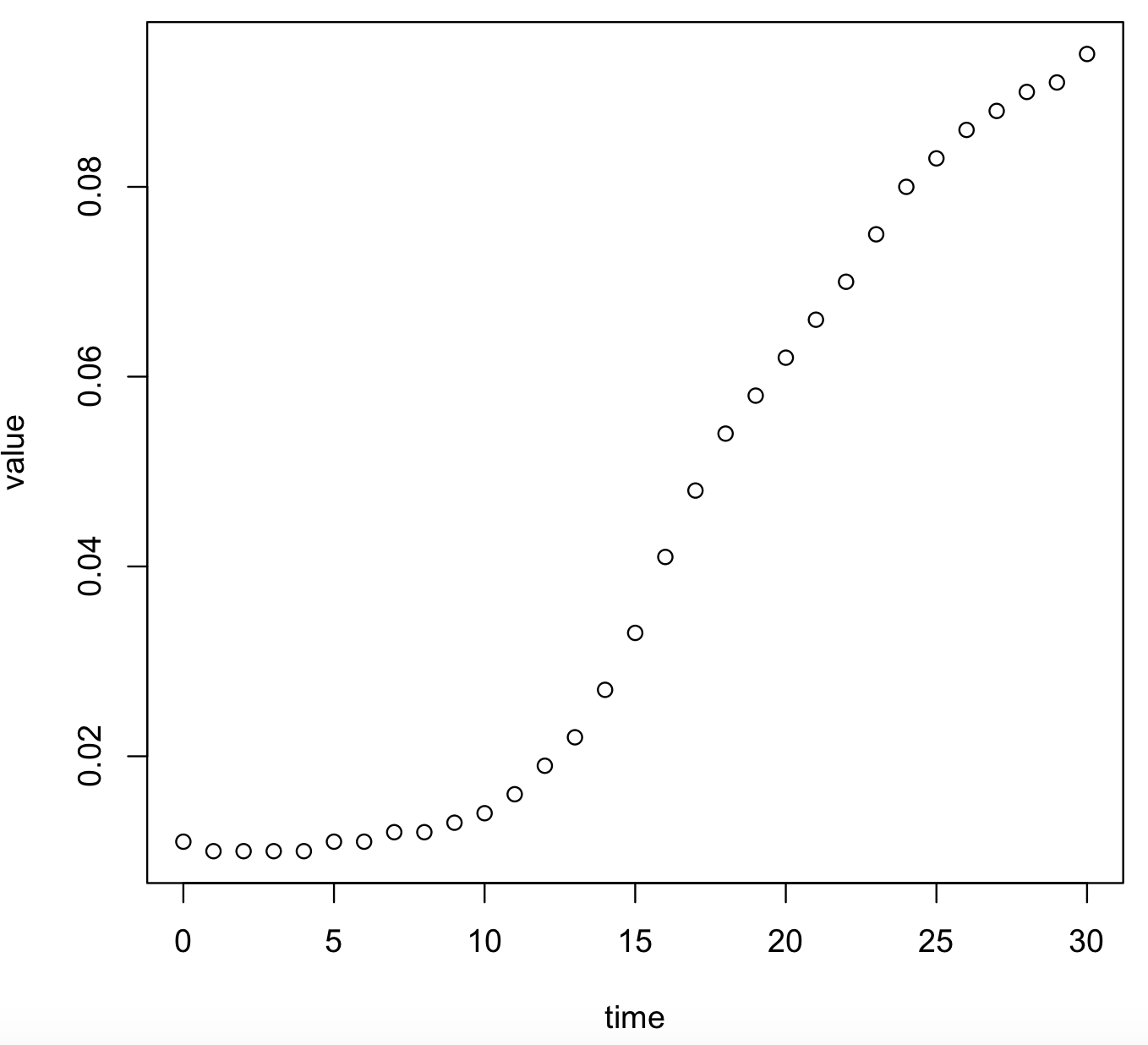
We can fit an exponential curve using the function drm() of the package drc. Notice that the type of curve will depend on its parametrization as indicated by the argument fct =. In this case is fct = G.4() or , for more information check drc manual and this page.
## fct for exponential growth
model_bactgrowth_strain_T <- drc::drm(value ~ time, fct = G.4(), data = bactgrowth_strain_T)
summary(model_bactgrowth_strain_T)
#Model fitted: Gompertz (4 parms)
#
#Parameter estimates:
#
#                Estimate Std. Error t-value   p-value
#b:(Intercept) -0.1799145  0.0061157 -29.419 < 2.2e-16 ***
#c:(Intercept)  0.0105954  0.0003694  28.683 < 2.2e-16 ***
#d:(Intercept)  0.1008913  0.0013430  75.122 < 2.2e-16 ***
#e:(Intercept) 16.6860271  0.1201873 138.833 < 2.2e-16 ***
#---
#Signif. codes:  0 ‘***’ 0.001 ‘**’ 0.01 ‘*’ 0.05 ‘.’ 0.1 ‘ ’ 1
#
#Residual standard error:
#
#0.001105757 (27 degrees of freedom)

## we can plot the fit of this function
plot(model_bactgrowth_strain_T)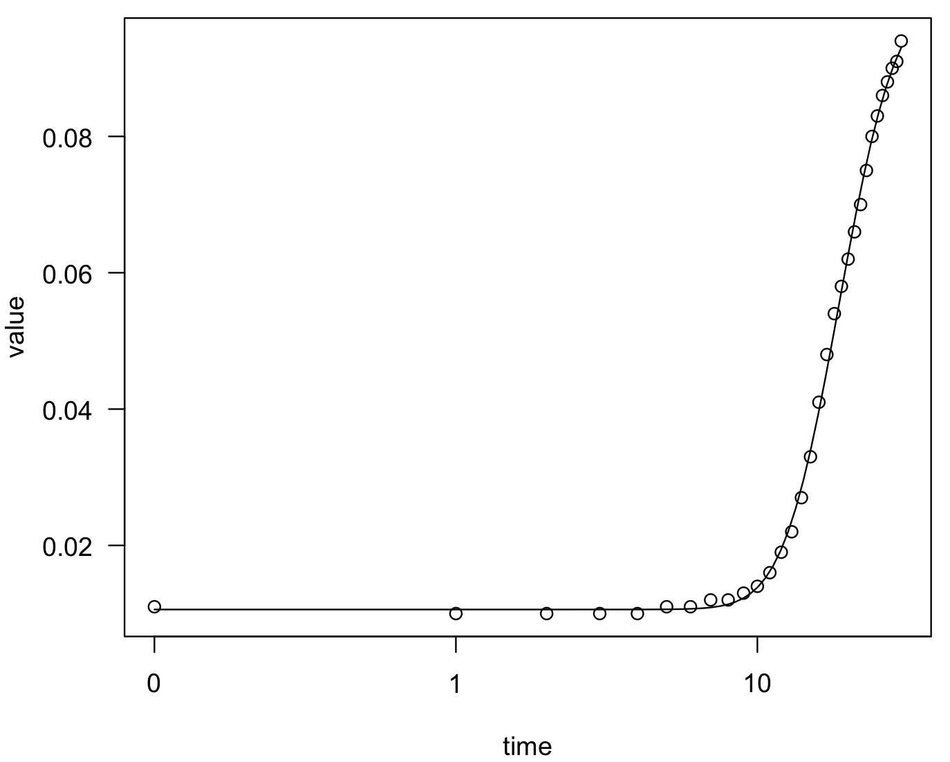
We can also estimate new values of growth of the bacteria strain T (dependent) for new time (predictor) using the function predict().
new_time <- data.frame(time = c(31,50,100,1000))
rownames(new_time) <- c("time_31", "time_50", "time_100", "time_1000")
new_values_growth <- predict(model_bactgrowth_strain_T, new_time)
names(new_values_growth) <- c("time_31", "time_50", "time_100", "time_1000")
new_values_growth
#  time_31   time_50  time_100 time_1000
#0.0942721 0.1006664 0.1008913 0.1008913
Like most non-linear models, it requires some parametrization determined by the curve that you observe by plotting your data. Another useful function is nls().
We can fit a exponential growth to our bactgrowth_strain_T using nls().
model_bactgrowth_strain_T_nls <- nls(value ~ a*exp(r*time), data = bactgrowth_strain_T,start = list(a = 0.5, r = 0.2))
summary(model_bactgrowth_strain_T_nls)
#Formula: value ~ a * exp(r * time)
#
#Parameters:
# Estimate Std. Error t value Pr(>|t|)
#a 0.011133 0.001356 8.213 4.69e-09 ***
#r 0.076416 0.004887 15.636 1.15e-15 ***
#---
#Signif. codes: 0 ‘***’ 0.001 ‘**’ 0.01 ‘*’ 0.05 ‘.’ 0.1 ‘ ’ 1
#
#Residual standard error: 0.008326 on 29 degrees of freedom
#
#Number of iterations to convergence: 11
#Achieved convergence tolerance: 3.249e-06
coef(model_bactgrowth_strain_T_nls)
# a r
#0.01113342 0.07641632
model_coeff <- coef(model_bactgrowth_strain_T_nls)
# plot this graph
plot(value ~ time, data = bactgrowth_strain_T, main = "bactgrowth_strain_T")
lines(bactgrowth_strain_T$time, model_coeff[1]*exp(model_coeff[2]*bactgrowth_strain_T$time), col = "orange2", lwd = 2)
# this is the same graph
#plot(value ~ time, data = bactgrowth_strain_T, main = "bactgrowth_strain_T")
#lines(bactgrowth_strain_T$time, 0.01113342*exp(0.07641632*bactgrowth_strain_T$time), col = "orange2", lwd = 2)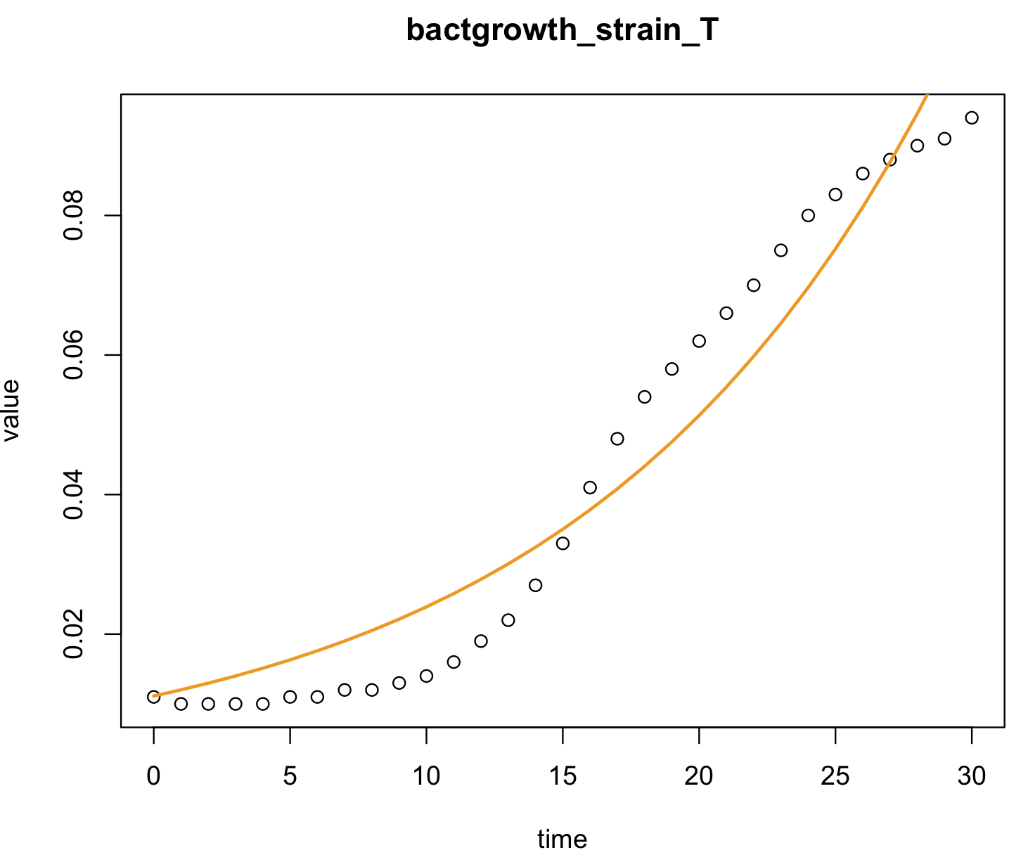 We can also estimate new values of growth of the bacteria strain T (dependent) for new time (predictor) using the function
 predict().
new_time <- data.frame(time = c(31,50,100,1000))
rownames(new_time) <- c("time_31", "time_50", "time_100", "time_1000")
new_values_growth_nls <- predict(model_bactgrowth_strain_T_nls, new_time)
names(new_values_growth_nls) <- c("time_31", "time_50", "time_100", "time_1000")
new_values_growth_nls
#       time_31      time_50     time_100    time_1000
#1.189684e-01 5.081454e-01 2.319249e+01 1.713226e+31
7.12 Toy datasets for regressions
Now that you have an illustrated example of regressions, you can choose among the following examples to do one of each exercise (e.g., linear regression, selecting predictors, logistic regressions, and non-linear regressions):
a) R-package ade4 dataset aravo for distribution of Alpine plants in Aravo (Valloire, France).
install.packages("ade4")
library(ade4)
data(aravo)
aravo_traits <- aravo$traits
head(aravo_traits)
#          Height Spread Angle  Area Thick  SLA N_mass Seed
#Agro.rupe      6     10    80  60.0  0.12  8.1 218.70 0.08
#Alop.alpi      5     20    20 190.9  0.20 15.1 203.85 0.21
#Anth.nipp     15      5    50 280.0  0.08 18.0 219.60 0.54
#Heli.sede      0     30    80 600.0  0.20 10.6 233.20 1.72
#Aven.vers     12     30    60 420.0  0.14 12.5 156.25 1.17
#Care.rosa     30     20    80 180.0  0.40  6.5 208.65 1.68
b) R-package ade4 dataset bacteria for total number of the 21 amino acids in 43 species of bacteria.
install.packages("ade4")
library(ade4)
data(bacteria)
bacteria_espaa <- bacteria$espaa
head(bacteria_espaa)
#          Ala   Arg   Asn   Asp  Cys   Gln   Glu   Gly   His   Ile    Leu   Lys   Met   Phe   Pro   Ser  Stp   Thr   Trp   Tyr   Val
#AERPECG 60384 48823 12907 24567 5896 12058 41892 54161 12189 32902  72081 22335 12476 17397 40897 47682 2619 29697  8324 21272 55421
#AQUAECG 28326 23565 17294 20754 3770  9791 46216 32425  7430 35203  50946 45092  8979 24736 19580 23036 1490 20221  4495 19887 38211
#ARCFUCG 50661 36713 20664 31358 7358 11448 56642 46562  9733 46172  60810 43489 16109 29467 24835 35350 2088 26833  6639 23426 55527
#BACHDCG 85555 55731 41785 58649 8393 47325 90358 81279 27972 80022 115667 67022 30743 51345 44287 64903 3558 64274 13156 39079 86451
#BACSUCG 91276 48698 46474 61327 9340 45257 85399 82164 26892 87050 114745 82768 31755 53186 43835 74444 3628 64270 12238 41133 80173
#BORBUCG 12555  8898 20318 14526 1822  6305 18931 14559  3403 29993  29020 28498  5008 17514  7044 20862  773 11018  1404 11814 14980
c) R-package ade4 dataset carni19 for carnivores body size and range.
install.packages("ade4")
library(ade4)
data(carni70)
carni70_size_range <- carni70$tab
head(carni70_size_range)
#                         size range
#Puma_concolor           37.01 36.00
#Herpailurus_yaguaroundi  2.59 24.00
#Leopardus_wiedii         3.20 21.75
#Leopardus_pardalis       7.90 24.50
#Oreailurus_jacobita      3.99  1.75
#Oncifelis_colocolo       2.99  6.25
d) R-package ade4 dataset cnc2003 for a data frame about cinema attendanace in France. This data frame contains the following variables, popuis the population department in million inhabitants. entris the number of movie theater visitors in million. receis the takings from ticket offices. seanis the number of proposed shows in thousands. commis the number of equipped communes in movie theaters (units). etabis the number of active movie theaters (units). salleis the number of active screens. fautis the number of proposed seats. artesis the number of movie theaters offering Art and Essay movies. multiis the number of active multiplexes. departis the name of the department. regis the administrative region of the department.
install.packages("ade4")
library(ade4)
data(cnc2003)
cnc2003_data <- cnc2003
head(cnc2003_data)
#     popu  entr   rece sean comm etab salle  faut artes multi                   depart                       reg
#D1 0.515 0.769  4.065   26   16   20    35  6288    12     0                      Ain               Rhone-Alpes
#D2 0.536 0.731  3.942   28   14   15    38  7403     8     0                    Aisne                  Picardie
#D3 0.345 0.499  2.789   17    7   11    28  3956     4     0                   Allier                  Auvergne
#D4 0.140 0.453  2.262   17   13   15    23  3480     7     0 Alpes de Hautes Provence Provence-Alpes-Coted'Azur
#D5 0.121 0.522  2.908   21   19   23    35  6053     5     0             Hautes Alpes Provence-Alpes-Coted'Azur
#D6 1.011 3.520 21.731  111   23   42    94 16764     8     1          Alpes Maritimes Provence-Alpes-Coted'Azur
e) R-package mlbench dataset PimaIndiansDiabetes2 for a data frame with 768 observations on 10 variables for the Pima Indians Diabetes Database: pregnant Number of times pregnant; glucose Plasma glucose concentration (glucose tolerance test); pressure Diastolic blood pressure (mm Hg); triceps Triceps skin fold thickness (mm); insulin 2-Hour serum insulin (mu U/ml); mass Body mass index (weight in kg/(height in m)^2); pedigree Diabetes pedigree function; age Age (years); diabetes Class variable (test for diabetes); prob_diabetes probability of diabetes (1 = yes, 0 = no).
install.packages("mlbench")
library(mlbench)
data(PimaIndiansDiabetes2)
PimaIndiansDiabetes2 <- na.omit(PimaIndiansDiabetes2)
PimaIndiansDiabetes2$prob_diabetes <- ifelse(PimaIndiansDiabetes2$diabetes == "pos", 1, 0)
head(PimaIndiansDiabetes2)
#    pregnant glucose pressure triceps insulin mass pedigree age diabetes prob_diabetes
#4         1      89       66      23      94 28.1    0.167  21      neg             0
#5         0     137       40      35     168 43.1    2.288  33      pos             1
#7         3      78       50      32      88 31.0    0.248  26      pos             1
#9         2     197       70      45     543 30.5    0.158  53      pos             1
#14        1     189       60      23     846 30.1    0.398  59      pos             1
#15        5     166       72      19     175 25.8    0.587  51      pos             1
f) R-package mlbench dataset BostonHousing for Housing data for 506 census tracts of Boston from the 1970 census. Variables include crim per capita crime rate by town; zn proportion of residential land zoned for lots over 25,000 sq.ft; indus proportion of non-retail business acres per town; chas Charles River dummy variable (= 1 if tract bounds river; 0 otherwise); nox nitric oxides concentration (parts per 10 million)rmaverage number of rooms per dwelling; age proportion of owner-occupied units built prior to 1940; dis weighted distances to five Boston employment centres; rad index of accessibility to radial highways; tax full-value property-tax rate per USD 10,000; ptratio pupil-teacher ratio by town; b 1000(B−0.63)2whereBis the proportion of blacks by town; lstat percentage of lower status of the population; medv median value of owner-occupied homes in USD 1000’s.
install.packages("mlbench")
library(mlbench)
data(BostonHousing)
BostonHousing_data <- BostonHousing
head(BostonHousing_data)
#     crim zn indus chas   nox    rm  age    dis rad tax ptratio      b lstat medv
#1 0.00632 18  2.31    0 0.538 6.575 65.2 4.0900   1 296    15.3 396.90  4.98 24.0
#2 0.02731  0  7.07    0 0.469 6.421 78.9 4.9671   2 242    17.8 396.90  9.14 21.6
#3 0.02729  0  7.07    0 0.469 7.185 61.1 4.9671   2 242    17.8 392.83  4.03 34.7
#4 0.03237  0  2.18    0 0.458 6.998 45.8 6.0622   3 222    18.7 394.63  2.94 33.4
#5 0.06905  0  2.18    0 0.458 7.147 54.2 6.0622   3 222    18.7 396.90  5.33 36.2
#6 0.02985  0  2.18    0 0.458 6.430 58.7 6.0622   3 222    18.7 394.12  5.21 28.7
7.13 ANOVA
An analysis of variance (ANOVA) will help you to determine if a dependent variable change according to the levels of one or more categorical independent variables. As part of this test, ANOVA will determine if a particular group has a different mean from the overall mean value of the data. This is determined by checking the variance of each of these individual groups against the overall variance of all the data. A significant result is reported if one or more groups falls outside the range of variation predicted (i.e., a null hypothesis that all groups have equal means).
In other words, ANOVA will test a null hypothesis (H0) that indicates a no difference in means versus the alternative (Ha) that indicates that the means are different between groups.
7.14 One-way ANOVA
The most common types of ANOVA include a one-way ANOVA with one independent variable and a two-way ANOVA with two independent variables. In order to perform an ANOVA, we use the function aov().
For an example of one-way ANOVA, we will continue using the crab_dataset
## we have already downloaded MASS and we assign the crabs dataset to an object
library(MASS)
?crabs
crab_dataset <- crabs
head(crab_dataset)
#  sp sex index   FL  RW   CL   CW  BD
#1  B   M     1  8.1 6.7 16.1 19.0 7.0
#2  B   M     2  8.8 7.7 18.1 20.8 7.4
#3  B   M     3  9.2 7.8 19.0 22.4 7.7
#4  B   M     4  9.6 7.9 20.1 23.1 8.2
#5  B   M     5  9.8 8.0 20.3 23.0 8.2
#6  B   M     6 10.8 9.0 23.0 26.5 9.8
We notice two categorical variables sp for species as “B” or “O” for blue or orange and sex for “M” males and “F” females.
For one-way ANOVA, we will determine if species variable sp that includes two categories or groups “B” or “O” have different means for the continuous variable CL or the carapace length (mm). We will use functions aov() and summary()
CL_anova_one_way <- aov(CL ~ sp, data = crab_dataset)
CL_anova_one_way
#Call:
#   aov(formula = CL ~ sp, data = crab_dataset)
#
#Terms:
#                      sp Residuals
#Sum of Squares   838.451  9246.853
#Deg. of Freedom        1       198
#
#Residual standard error: 6.833833
#Estimated effects may be unbalanced
summary(CL_anova_one_way)
#             Df Sum Sq Mean Sq F value   Pr(>F)
#sp            1    838   838.5   17.95 3.47e-05 ***
#Residuals   198   9247    46.7
#---
#Signif. codes:  0 ‘***’ 0.001 ‘**’ 0.01 ‘*’ 0.05 ‘.’ 0.1 ‘ ’ 1
Overall, the Pr(>F) column provides the p-value (significance) of the F-statistic, which is very low (p < 0.0001).
These results suggest that the we did find little support for the null hypothesis of no difference among group means of sp (i.e., species “B” or “O”) based on CL or the carapace length size (mm).
Therefore, the measurements of carapace length seem to be different between the two species of crabs studied.
7.15 Two-way ANOVA
We can perform a two-way ANOVA by including two independent variables. For a two-way ANOVA, we will both categorical variables sp for species as “B” or “O” for blue or orange and sex for “M” males and “F” females. As a dependent, we will use again the continuous variable CL or the carapace length (mm). We will use functions aov() and summary()
CL_anova_two_way <- aov(CL ~ sp + sex, data = crab_dataset)
CL_anova_two_way
#Call:
#   aov(formula = CL ~ sp + sex, data = crab_dataset)
#
#Terms:
#                      sp      sex Residuals
#Sum of Squares   838.451  111.154  9135.699
#Deg. of Freedom        1        1       197
#
#Residual standard error: 6.809854
#Estimated effects may be unbalanced
summary(CL_anova_two_way)
#             Df Sum Sq Mean Sq F value   Pr(>F)
#sp            1    838   838.5  18.080 3.27e-05 ***
#sex           1    111   111.2   2.397    0.123
#Residuals   197   9136    46.4
#---
#Signif. codes:  0 ‘***’ 0.001 ‘**’ 0.01 ‘*’ 0.05 ‘.’ 0.1 ‘ ’ 1
Overall, the Pr(>F) column provides two p-values
(i.e., p = 3.27e-05 and p = 0.123 ) for the corresponding F-statistic (i.e., 18.080 and 2.397) and, again, only the species type (variable sp) shows evidence of difference among group means of their CL or the carapace length (mm). In contrast, the gender of the crabs (variable sex) does not explain differences in the measurements of carapace length.
7.16 ANOVA Post-hoc tests
We can perform a post-hoc test to find the differences among group means. One of such tests is Tukey’s Honestly Significant Difference (Tukey’s HSD) for pairwise comparisons.
We use the function TukeyHSD() on the resulting ANOVA object.
## one-way ANOVA
TukeyHSD(CL_anova_one_way)
#  Tukey multiple comparisons of means
#    95% family-wise confidence level
#
#Fit: aov(formula = CL ~ sp, data = crab_dataset)
#
#$sp
#     diff      lwr      upr    p adj
#O-B 4.095 2.189144 6.000856 3.47e-05

## two-way ANOVA
TukeyHSD(CL_anova_two_way)
#  Tukey multiple comparisons of means
#    95% family-wise confidence level
#
#Fit: aov(formula = CL ~ sp + sex, data = crab_dataset)
#
#$sp
#     diff      lwr      upr    p adj
#O-B 4.095 2.195772 5.994228 3.27e-05
#
#$sex
#     diff        lwr      upr    p adj
#M-F 1.491 -0.4082279 3.390228 0.123181
Again, these results support that the variable sp for species as “B” or “O” is important when comparing means of CL or the carapace length (mm) of these crabs.
7.17 Beyond ANOVA: Kruskal-Wallis Test
Some samples that you want to compare might have a non-normal or unknown distributions. In this case, you can use non-parametric methods like Kruskal-Wallis Test to determine if samples have different medians. The null hypothesis is that the medians of all groups are all equal, while the alternative hypothesis is that at least one sample median is different from the median of at least one other group or sample.
We can reuse the crabs dataset from the package ‘MASS’ – IMPORTANT: this test does not assume normality.
## we can get crabs dataset
library(MASS)
crab_dataset <- crabs
head(crab_dataset)
#  sp sex index   FL  RW   CL   CW  BD
#1  B   M     1  8.1 6.7 16.1 19.0 7.0
#2  B   M     2  8.8 7.7 18.1 20.8 7.4
#3  B   M     3  9.2 7.8 19.0 22.4 7.7
#4  B   M     4  9.6 7.9 20.1 23.1 8.2
#5  B   M     5  9.8 8.0 20.3 23.0 8.2
#6  B   M     6 10.8 9.0 23.0 26.5 9.8
We can implement this Kruskal-Wallis Test using the function kruskal.test() for CL carapace length (mm) as dependent and grouping by sex or species.
## for sex as grouping
kruskal.test(CL ~ sex, data = crab_dataset)
#   Kruskal-Wallis rank sum test
#
#data:  CL by sex
#Kruskal-Wallis chi-squared = 1.8424, df = 1, p-value = 0.1747

## for species as grouping
kruskal.test(CL ~ sp, data = crab_dataset)
#   Kruskal-Wallis rank sum test
#
#data:  CL by sp
#Kruskal-Wallis chi-squared = 15.698, df = 1, p-value = 7.431e-05
These results agree with the one-way ANOVA results.
7.18 Toy datasets for ANOVA
Now that you have examples of ANOVA, you can choose among the following examples for further examples
a) R-package agridat dataset fisher.barley for results of trials of 5 varieties of barley were conducted at 6 stations in Minnesota during the years 1931-1932. This result in a data frame with 60 observations on the following 4 variables: yield yield, bu/ac; gen genotype/variety, 5 levels; env environment/location, 2 levels; year year, 1931/1932.
install.packages("agridat")
library(agridat)
data(fisher.barley)
fisher_barley <- fisher.barley
head(fisher_barley)
#  yield       gen            env year
#1  81.0 Manchuria UniversityFarm 1931
#2  80.7 Manchuria UniversityFarm 1932
#3 146.6 Manchuria         Waseca 1931
#4 100.4 Manchuria         Waseca 1932
#5  82.3 Manchuria         Morris 1931
#6 103.1 Manchuria         Morris 1932
b) R-package agridat dataset gumpertz.pepper for results with 800 observations on the following 6 variables: field field factor, 2 levels; row x ordinate; quadrat y ordinate; disease presence (Y) or absence (N) of disease; water soil moisture percent; leaf leaf assay count. Each field is 20 rows by 20 quadrates, with 2 to 3 bell pepper plants per plot. If any plant was wilted, dead, or had lesions, the Phytophthora disease was considered to be present in the plot. The soil pathogen load was assayed as the number of leaf disks colonized out of five. In field 2, the pattern of disease presence appears to follow soil water content. In field 1, no obvious trends were present.
install.packages("agridat")
library(agridat)
data(gumpertz.pepper)
gumpertz_pepper <- gumpertz.pepper
head(gumpertz_pepper)
#  field row quadrat disease water leaf
#1    F1   1       1       N 15.05    5
#2    F1   1       2       N 14.32    2
#3    F1   1       3       N 13.99    3
#4    F1   1       4       N 13.85    0
#5    F1   1       5       N 13.16    5
#6    F1   1       6       N 11.81    5