Session 8 – Multidimensional Data in R
Many datasets derive from multiple variables measured from hundreds of individuals and many of such parameters are obtained simultaneously (i.e., multidimensional) and together are often difficult to interpret. Most researchers aim to reduce such complexity, identify groups of interest or increase data interpretability using diverse methods like principal component analysis (PCA), multidimensional scaling (MDS), cluster analyses among others. We will explore some of these methods.
8.1 Principal Component Analysis
PCA is a common approach to reduce dimensionality in a dataset. For instance, PCA reduce the data complexity from many variables into few summary components, while preserving much of the statistical information. During the analysis, new variables (named components) are found that are linear functions of those in the original dataset, that successively maximize variance and that are uncorrelated with each other, see Jolliffe and Cadima 2016.
PCA is recommended when you have large dataset of variables (e.g., > 8) and many individuals (>20 or better in the hundreds) with measurements of such variables. For this example, we will use the env data frame of the doubs dataset from the R-package ade4. The env is a data frame with 30 rows (sites) and 11 environmental variables.
## we can install ade4 and load the dataset for this example
install.packages("ade4")
library(ade4)

##load the doubs dataset into the R environment
data(doubs)

## dataset of ecological tables for environmental variables, fish species and spatial coordinates for 30 sites.
?doubs

## we will use only the environmental variables
env_raw <- doubs$env
head(env_raw)
#  dfs alt   slo flo pH har pho nit amm oxy bdo
#1   3 934 6.176  84 79  45   1  20   0 122  27
#2  22 932 3.434 100 80  40   2  20  10 103  19
#3 102 914 3.638 180 83  52   5  22   5 105  35
#4 185 854 3.497 253 80  72  10  21   0 110  13
#5 215 849 3.178 264 81  84  38  52  20  80  62
#6 324 846 3.497 286 79  60  20  15   0 102  53
We can start by getting a pairwise bivariate plots of these 11 variables.
## we can install ade4 and load the dataset for this example
pairs(env_raw, pch = 19, cex=0.5)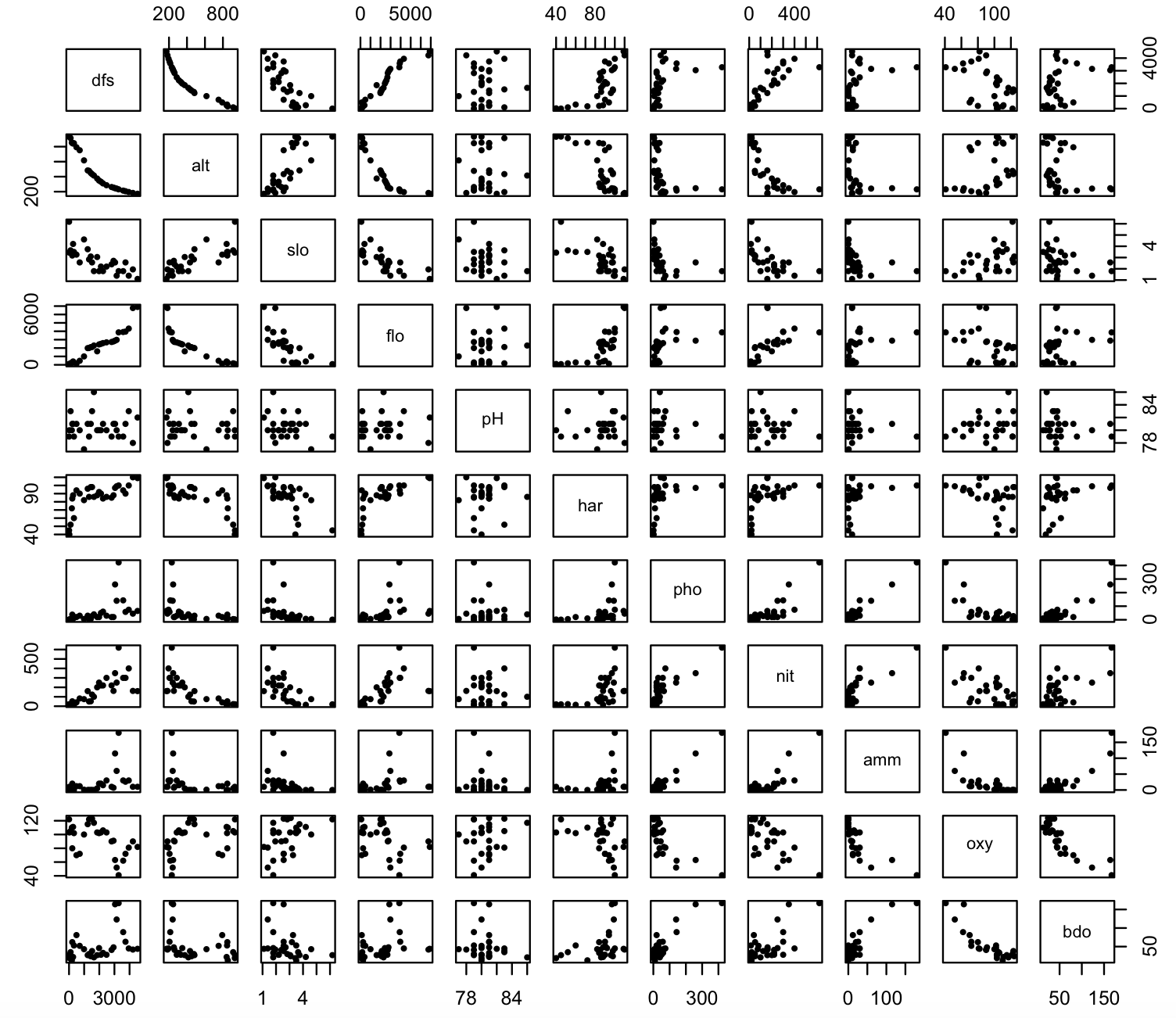
We notice a relative variability in these pairwise plots. Some show a linear relationship, others do not. Likewise, some scales differences are evident (some are in the hundreds, others much less).
## we can use the function modify() form the R-package **purrr** to standardize this dataset using log
library(purrr)
env_log <- purrr::modify(env_raw, log)
head(env_log)
#       dfs      alt      slo      flo       pH      har       pho      nit      amm      oxy      bdo
#1 1.098612 6.839476 1.820671 4.430817 4.369448 3.806662 0.0000000 2.995732     -Inf 4.804021 3.295837
#2 3.091042 6.837333 1.233726 4.605170 4.382027 3.688879 0.6931472 2.995732 2.302585 4.634729 2.944439
#3 4.624973 6.817831 1.291434 5.192957 4.418841 3.951244 1.6094379 3.091042 1.609438 4.653960 3.555348
#4 5.220356 6.749931 1.251905 5.533389 4.382027 4.276666 2.3025851 3.044522     -Inf 4.700480 2.564949
#5 5.370638 6.744059 1.156252 5.575949 4.394449 4.430817 3.6375862 3.951244 2.995732 4.382027 4.127134
#6 5.780744 6.740519 1.251905 5.655992 4.369448 4.094345 2.9957323 2.708050     -Inf 4.624973 3.970292

## Notice some -Inf value, we will remove that column 9 that corresponds to ‘amm’
env_log_red <- env_log[,-9]
head(env_log_red)
#       dfs      alt      slo      flo       pH      har       pho      nit      oxy      bdo
#1 1.098612 6.839476 1.820671 4.430817 4.369448 3.806662 0.0000000 2.995732 4.804021 3.295837
#2 3.091042 6.837333 1.233726 4.605170 4.382027 3.688879 0.6931472 2.995732 4.634729 2.944439
#3 4.624973 6.817831 1.291434 5.192957 4.418841 3.951244 1.6094379 3.091042 4.653960 3.555348
#4 5.220356 6.749931 1.251905 5.533389 4.382027 4.276666 2.3025851 3.044522 4.700480 2.564949
#5 5.370638 6.744059 1.156252 5.575949 4.394449 4.430817 3.6375862 3.951244 4.382027 4.127134
#6 5.780744 6.740519 1.251905 5.655992 4.369448 4.094345 2.9957323 2.708050 4.624973 3.970292

## dataset of ecological tables for environmental variables, fish species and spatial coordinates for 30 sites.
?doubs

## we can install ade4 and load the modified dataset for this example
pairs(env_log_red, pch = 19, cex=0.5)
We can run PCA using the preloaded function in R or with several specialized packages. We will start with the functions prcomp() and summary().
## apply PCA - scale. = TRUE is highly advisable, but default is FALSE.
env_prcomp <- prcomp(env_log_red, center = TRUE, scale. = TRUE)
env_prcomp
#Standard deviations (1, .., p=10):
# [1] 2.5031260 1.2651443 0.9875811 0.6860815 0.5095091 0.3946341 0.3212448 0.2824013 0.2580574 0.1512203
#
#Rotation (n x k) = (10 x 10):
#            PC1         PC2        PC3         PC4          PC5         PC6          PC7         PC8         PC9         PC10
#dfs  0.36486258 -0.18617302  0.1482270 -0.27425018  0.070856291 -0.06822936  0.375972370  0.04774989 -0.73277048  0.211581601
#alt -0.36451449  0.12764399 -0.1690422 -0.36872511  0.165563399  0.30103670  0.159545574  0.45954368 -0.16927250 -0.550436218
#slo -0.33426066  0.15461463  0.2062596 -0.41599181 -0.694152941  0.08059586 -0.008314283 -0.38539136 -0.10748520  0.016710642
#flo  0.35536702 -0.26645120  0.2469480  0.07962110 -0.140470255 -0.21095156  0.148040510 -0.22735329  0.11111159 -0.764991160
#pH   0.02686455 -0.43046956 -0.8301590 -0.07333534 -0.270021833 -0.14147519 -0.099820286 -0.07667608 -0.09705901 -0.035234427
#har  0.32775459 -0.15043755  0.1025784 -0.71869778  0.192865111 -0.02065425 -0.450542106  0.06200716  0.30538254  0.071982806
#pho  0.35978479  0.15025127 -0.2384279 -0.09780973  0.004998182  0.59283974  0.493290882 -0.25929815  0.33522306  0.084468872
#nit  0.36509191 -0.03139547  0.1053406  0.23840435 -0.511528294  0.41078684 -0.313263865  0.51006660 -0.09509725 -0.006021563
#oxy -0.25192228 -0.56073462  0.2173434 -0.06473107 -0.174757541 -0.08405657  0.438140938  0.36832297  0.39110186  0.229102408
#bdo  0.24827761  0.55517993 -0.1762335 -0.13016095 -0.252295130 -0.55318468  0.254587830  0.33694829  0.18286003  0.026082994

## dataset of ecological tables for environmental variables, fish species and spatial coordinates for 30 sites.
?doubs
The output of env_prcomp includes the standard deviation of each of the 10 principal components (PCs). You should expect as many PCs as the number of variables in your dataset (i.e., 10 variables, 10 PCs). The values under Rotation (n x k) are the loadings of each of the variables in each component (PC) and provide information about how each variables contribute to their calculation. Loadings range from -1 to 1 and higher the absolute value of these loadings on a PC, the more that variable is related to that PC (i.e., it is better represented). Loadings with absolute values >0.4 are usually consider to have a strong relationship with that components. Notice the sign of the loading, some are positive, and some are negative. Positive is direct relationship, while a negative is an inverse relationship.
## we can see the structure of the analysis
str(env_prcomp)
#List of 5
# $ sdev    : num [1:10] 2.503 1.265 0.988 0.686 0.51 ...
#$ rotation: num [1:10, 1:10] 0.3649 -0.3645 -0.3343 0.3554 0.0269 ...
#  ..- attr(*, "dimnames")=List of 2
# .. ..$ : chr [1:10] "dfs" "alt" "slo" "flo" ...
#  .. ..$ : chr [1:10] "PC1" "PC2" "PC3" "PC4" ...
#$ center  : Named num [1:10] 6.887 6.019 0.943 7.153 4.388 ...
# ..- attr(*, "names")= chr [1:10] "dfs" "alt" "slo" "flo" ...
#$ scale   : Named num [1:10] 1.6786 0.5747 0.3863 1.3041 0.0214 ...
# ..- attr(*, "names")= chr [1:10] "dfs" "alt" "slo" "flo" ...
#$ x       : num [1:30, 1:10] -6 -4.96 -3.6 -3.18 -1.24 ...
#  ..- attr(*, "dimnames")=List of 2
#  .. ..$ : chr [1:30] "1" "2" "3" "4" ...
#  .. ..$ : chr [1:10] "PC1" "PC2" "PC3" "PC4" ...
# - attr(*, "class")= chr "prcomp"

## we can get a summary
summary(env_prcomp)
#Importance of components:
#                          PC1    PC2     PC3     PC4     PC5     PC6     PC7     PC8     PC9    PC10
#Standard deviation     2.5031 1.2651 0.98758 0.68608 0.50951 0.39463 0.32124 0.28240 0.25806 0.15122
#Proportion of Variance 0.6266 0.1601 0.09753 0.04707 0.02596 0.01557 0.01032 0.00798 0.00666 0.00229
#Cumulative Proportion 0.6266 0.7866 0.88415 0.93123 0.95719 0.97276 0.98308 0.99105 0.99771 1.00000Thesummary(env_prcomp) output describe the importance of each PC. The proportion of variance indicates the proportion of the total variance in the data explained by each PC. We can notice the values of the second row are progressively added resulting in a cumulative proportion of explained variance. In most cases, the first and second PC accounts for most of the variance explain (i.e., PC1 – 62.66% + PC2 – 16.01% = 78.66%). The rest of PCs are progressively less and less relevant to explain the variance of the data and they are usually ignored.
For most purposes, the first two PCs are used for plots and visualizing dimensionality reduction. However, we can determine how many PCs to retain using a scree plot and other references using the R-package factoextra.
We can get an scree plot with the function fviz_eig().
## install package, if not present. It also requires the R-package ggplot2.
install.packages("factoextra")
install.packages("ggplot2")
library(factoextra)
#Loading required package: ggplot2
#Welcome! Want to learn more? See two factoextra-related books at https://goo.gl/ve3WBa
factoextra::fviz_eig(env_prcomp)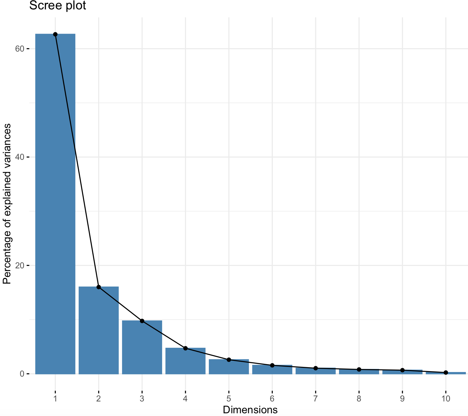
This scree plot shows the eigenvalues and these represent the total amount of variance that can be explained by a given principal component. For example, for PC1 its eigenvalue is 62.66%.Therefore, these plots provide information on the percentage of variances explained by each PC and support our intuition that the first two PCs are the most useful to summarize the variability of our dataset. For instance, we see a marked drop in the percentage of explained variance after PC2, and we can ignore the rest of PCs (3-10) that explain relatively little variation. Thus, we should focus primarily on PC1 and PC2.
We can graph our samples (i.e., individuals on our dataset) with their PC1 and PC2 coordinates using the function fviz_pca_ind().
factoextra::fviz_pca_ind(env_prcomp,
                   col.ind = "cos2",
             gradient.cols = c("firebrick4", "gray", "dodgerblue4"),
                     repel = TRUE)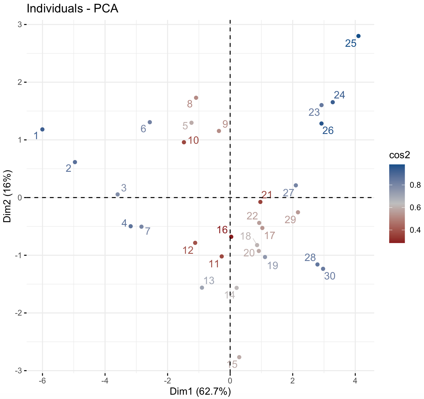
Individuals with a similar profile tend to group together and color cos2 refers to the quality of representation. Notice that you can choose the color gradient that you want with the argument gradient.cols, it might need 3 colors.
### NOTE: Sometimes you get this error.
#Error in UseMethod("depth") :
#  no applicable method for 'depth' applied to an object of class "NULL"
### Try to resubmit the fviz_pca_ind() after closing the graph window.
We can also graph of variables that we used in our PCA using the function fviz_pca_var().
## dataset of ecological tables for environmental variables, fish species and spatial coordinates for 30 sites.
?doubs
## plot
factoextra::fviz_pca_var(env_prcomp,
             col.var = "contrib",
             gradient.cols = c("dodgerblue4", "#E7B800", "firebrick4"),
             repel = TRUE)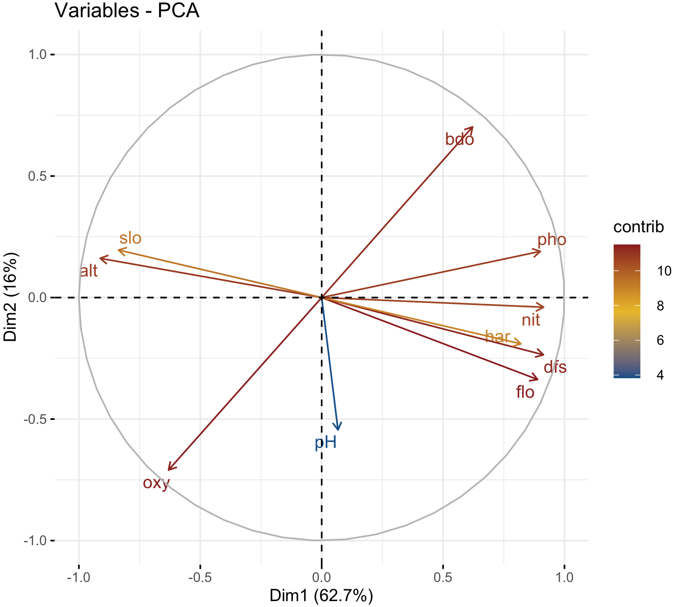
We can see that positive correlated variables point to the same side of the plot, while negative correlated variables point to opposite sides of the graph. Notice that you can choose the color gradient that you want with the argument gradient.cols, it might need 3 colors.
### NOTE: Sometimes you get this error.
#Error in UseMethod("depth") :
#  no applicable method for 'depth' applied to an object of class "NULL"
### Try to resubmit the fviz_pca_ind() after closing the graph window.
We can also graph plot both individuals and variables at the same time using the function fviz_pca_biplot().
factoextra::fviz_pca_biplot(env_prcomp,
                col.var = "gray", # Variables color
                col.ind = "dodgerblue4",  # Individuals color
                repel = TRUE)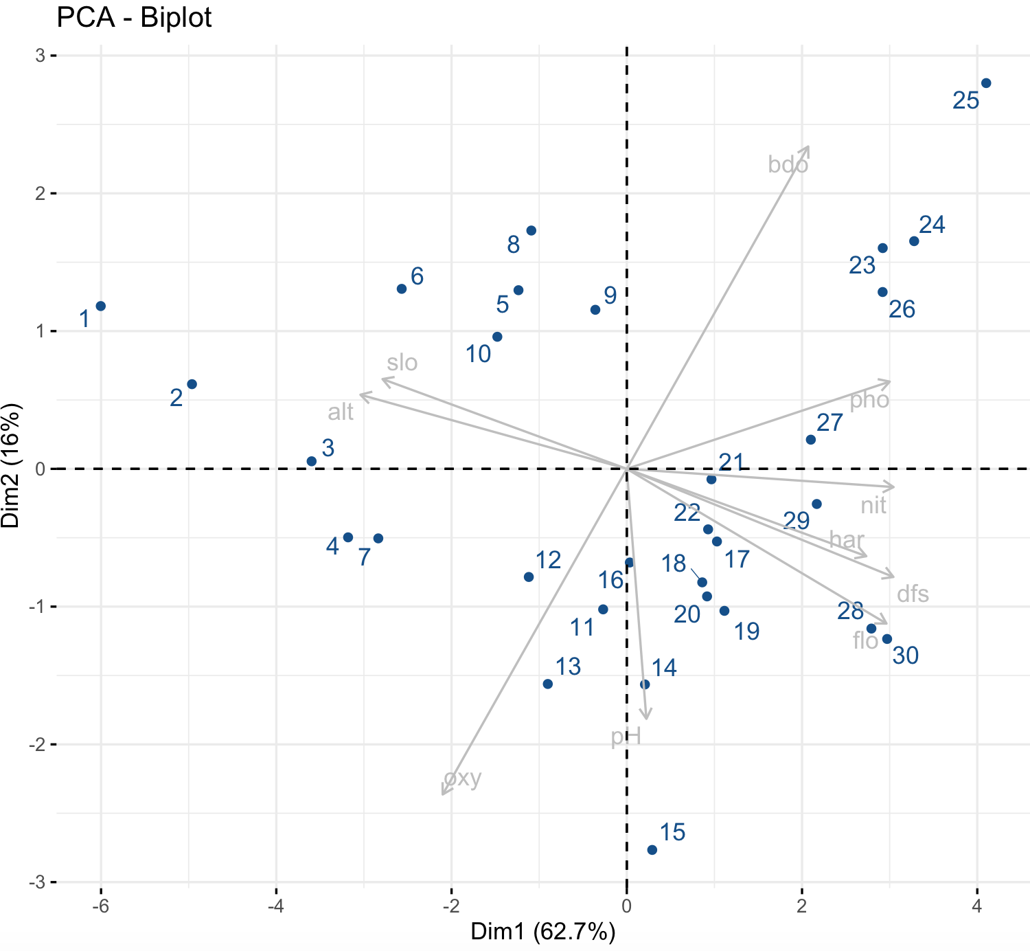
We can extract other metrics of our PCA with several functions of factoextra.
The eigenvalues can be printed with the function get_eigenvalue()describe the importance of each PC. Similar to summary(env_prcomp).
## Eigenvalues
eig_val_env_prcomp <- factoextra::get_eigenvalue(env_prcomp)
eig_val_env_prcomp
#       eigenvalue variance.percent cumulative.variance.percent
#Dim.1  6.26563999       62.6563999                    62.65640
#Dim.2  1.60059015       16.0059015                    78.66230
#Dim.3  0.97531642        9.7531642                    88.41547
#Dim.4  0.47070789        4.7070789                    93.12254
#Dim.5  0.25959955        2.5959955                    95.71854
#Dim.6  0.15573609        1.5573609                    97.27590
#Dim.7  0.10319822        1.0319822                    98.30788
#Dim.8  0.07975052        0.7975052                    99.10539
#Dim.9  0.06659361        0.6659361                    99.77132
#Dim.10 0.02286757        0.2286757                   100.00000
The variable results can be printed with the function get_pca_var().
## dataset of ecological tables for environmental variables, fish species and spatial coordinates for 30 sites.
?doubs

## Results for Variables
res_var_env_prcomp <- factoextra::get_pca_var(env_prcomp)
# Coordinates
res_var_env_prcomp$coord
# Contributions to the PCs
res_var_env_prcomp$contrib
# Quality of representation
res_var_env_prcomp$cos2
The individual (i.e., samples) associated results can be printed with the function get_pca_ind().
## Results for individuals
res_ind_env_prcomp <- factoextra::get_pca_ind(env_prcomp)
# Coordinates -- this is same as env_prcomp$x
res_ind_env_prcomp$coord
# Contributions to the PCs
res_ind_env_prcomp$contrib
# Quality of representation
res_ind_env_prcomp$cos2
8.2 Multidimensional scaling
We use multidimensional scaling helps to visualize similarities of individual cases or samples of a dataset. In this analysis, we reduce dimensions to be able to visualize or represent data points in a more friendly manner. We start with a set of samples or individuals measured on several numeric variables. After the analysis, we get a representation of the distances among these samples or individuals in a lower dimensional space (e.g., 2 dimensions), so we can infer the relative relationship (distance) between them. In other words, individuals or samples that are closer are more similar.
We will use our example `env_log_red, but we need to add names to the sites for visualization.
## dataset of ecological tables for environmental variables, fish species and spatial coordinates for 30 sites.
?doubs

## We can name our samples by assigned a unique row name.
env_log_red_MDS <- env_log_red
rownames(env_log_red_MDS) <- paste0("site_", 1:nrow(env_log_red_MDS))
head(env_log_red_MDS)
#            dfs      alt      slo      flo       pH      har       pho      nit      oxy      bdo
#site_1 1.098612 6.839476 1.820671 4.430817 4.369448 3.806662 0.0000000 2.995732 4.804021 3.295837
#site_2 3.091042 6.837333 1.233726 4.605170 4.382027 3.688879 0.6931472 2.995732 4.634729 2.944439
#site_3 4.624973 6.817831 1.291434 5.192957 4.418841 3.951244 1.6094379 3.091042 4.653960 3.555348
#site_4 5.220356 6.749931 1.251905 5.533389 4.382027 4.276666 2.3025851 3.044522 4.700480 2.564949
#site_5 5.370638 6.744059 1.156252 5.575949 4.394449 4.430817 3.6375862 3.951244 4.382027 4.127134
#site_6 5.780744 6.740519 1.251905 5.655992 4.369448 4.094345 2.9957323 2.708050 4.624973 3.970292
We can perform MDS using the function dis() and cmdscale()for metric or classical MDS with two dimensions k = 2.
## Classical MDS: N rows (objects) x p columns (variables)
# get Euclidean distances between the rows
env_log_red_MDS_d <- dist(env_log_red_MDS)
# k is the number of dimensions
env_log_red_MDS_fit <- cmdscale(env_log_red_MDS_d,eig=TRUE, k=2)
str(env_log_red_MDS_fit)
#List of 5
# $ points: num [1:30, 1:2] -7.21 -5.58 -3.84 -3.11 -1.83 ...
#  ..- attr(*, "dimnames")=List of 2
#  .. ..$ : chr [1:30] "site_1" "site_2" "site_3" "site_4" ...
#  .. ..$ : NULL
#$ eig   : num [1:30] 203.13 25.14 9.43 4.54 3.22 ...
#$ x     : NULL
#$ ac    : num 0
#$ GOF   : num [1:2] 0.92 0.92
We can plot this samples using the x-y coordinates in env_log_red_MDS_fit$points.
## plot solution
x <- env_log_red_MDS_fit$points[,1]
y <- env_log_red_MDS_fit$points[,2]
plot(x, y, xlab= "Coordinate 1 - MDS", ylab="Coordinate 2 - MDS", main="Metric MDS for env_log_red", type="n")
text(x, y, labels = row.names(env_log_red_MDS), cex=.7) 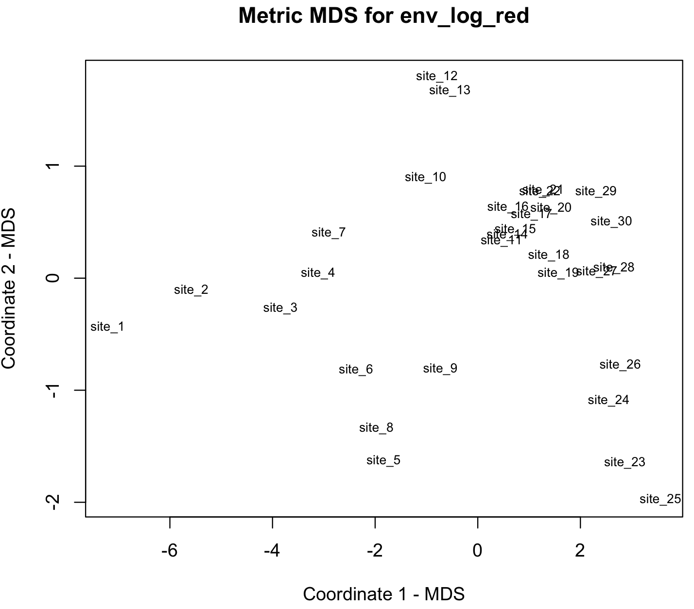
We use nonmetric multidimensional scaling to visualizing the function isoMDS() of the R-package MASS.
## For nonmetric MDS, we load MASS (we installed this package before)
library(MASS)
env_log_red_MDS_d <- dist(env_log_red_MDS)
env_log_red_NMDS <- MASS::isoMDS(env_log_red_MDS_d, k=2)
str(env_log_red_NMDS)
#List of 2
# $ points: num [1:30, 1:2] -7.64 -5.6 -3.74 -3.08 -1.72 ...
#  ..- attr(*, "dimnames")=List of 2
#  .. ..$ : chr [1:30] "site_1" "site_2" "site_3" "site_4" ...
#  .. ..$ : NULL
# $ stress: num 2.49

## plot solution NMDS solution
x <- env_log_red_NMDS$points[,1]
y <- env_log_red_NMDS$points[,2]
plot(x, y, xlab= "Coordinate 1 - NMDS", ylab="Coordinate 2 - NMDS", main="Nonmetric MDS for env_log_red", type="n")
text(x, y, labels = row.names(env_log_red_MDS), cex=.7) 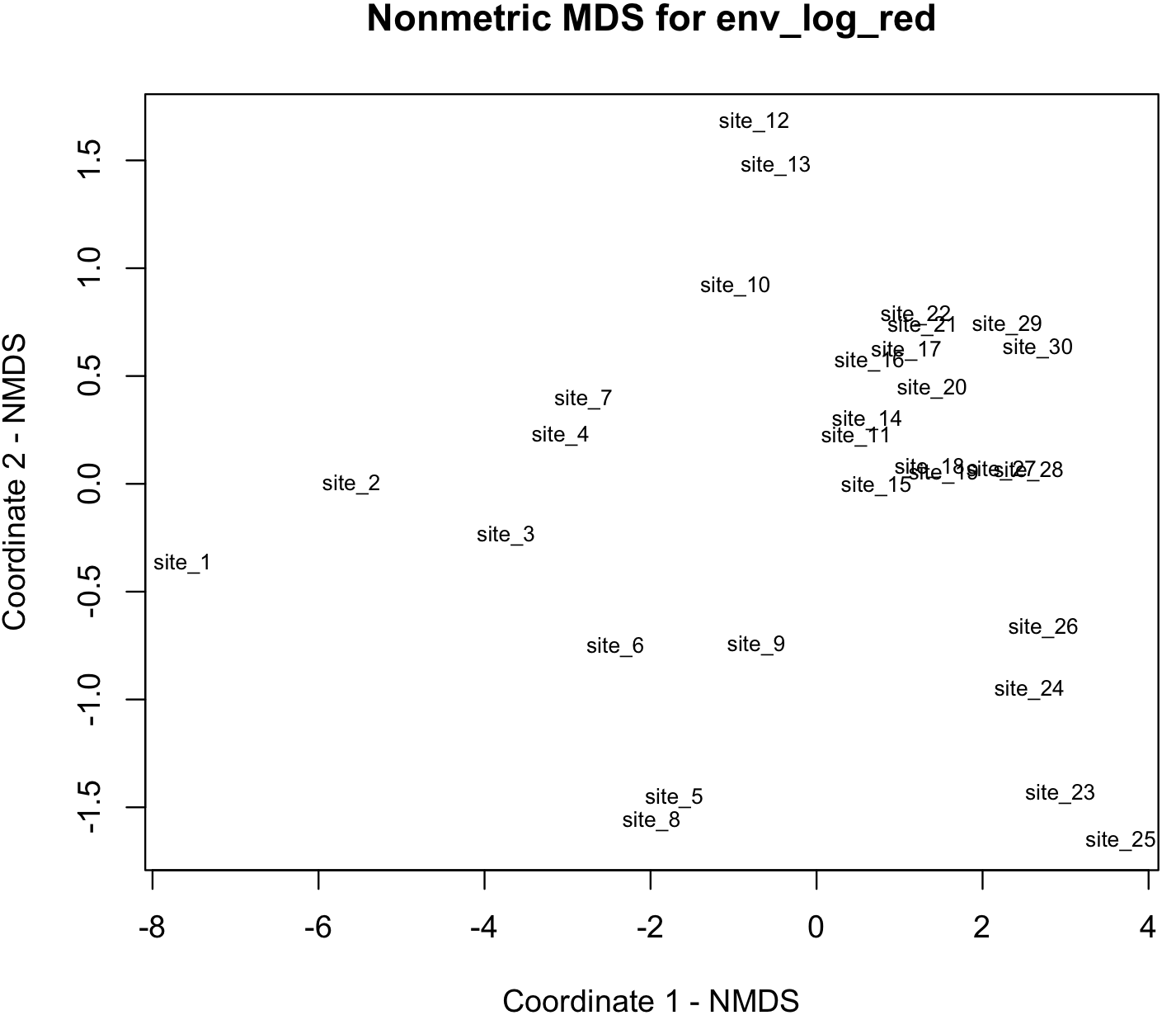
8.3 Cluster analysis: DFA
Many biological datasets might have an underlying structure were groups or clusters that can be outcome of a treatment. Finding those set of objects that are more similar might help to identify groups or clusters that can used to classification of other samples.
We use a classic example known as the Fisher’s or Anderson’s Iris data set, which is a dataset of multiple measurements introduced by Ronald Fisher to illustrate taxonomic problems as an example of linear discriminant analysis. This dataset consists of 50 samples of three species of flowers: Iris setosa, Iris virginica and Iris versicolor. The dataset includes four features of the flower measured in centimeters. This dataset can be loaded from the R-package datasets.
install.packages("datasets")
library(datasets)
data(iris)
?iris
iris_dataset <- iris

summary(iris_dataset)
#  Sepal.Length    Sepal.Width     Petal.Length    Petal.Width          Species
#Min.   :4.300   Min.   :2.000   Min.   :1.000   Min.   :0.100   setosa    :50
#1st Qu.:5.100   1st Qu.:2.800   1st Qu.:1.600   1st Qu.:0.300   versicolor:50
#Median :5.800   Median :3.000   Median :4.350   Median :1.300   virginica :50
#Mean   :5.843   Mean   :3.057   Mean   :3.758   Mean   :1.199
#3rd Qu.:6.400   3rd Qu.:3.300   3rd Qu.:5.100   3rd Qu.:1.800
#Max.   :7.900   Max.   :4.400   Max.   :6.900   Max.   :2.500
head(iris_dataset)
#  Sepal.Length Sepal.Width Petal.Length Petal.Width Species
#1          5.1         3.5          1.4         0.2  setosa
#2          4.9         3.0          1.4         0.2  setosa
#3          4.7         3.2          1.3         0.2  setosa
#4          4.6         3.1          1.5         0.2  setosa
#5          5.0         3.6          1.4         0.2  setosa
#6          5.4         3.9          1.7         0.4  setosa
We can perform discriminant function analysis (DFA) or Linear Discriminant Analysis (LDA) to find a function (e.g., linear classifier) to separate samples in to two or more classes. For this analysis, we will the function lda() from the package MASS.
## we have used the packages MASS and ggplot2.
library(MASS)
library(ggplot2)
## we get the names of predictors (i.e., measurements) and target group
str(iris_dataset)
#'data.frame':  150 obs. of  5 variables:
#$ Sepal.Length: num  5.1 4.9 4.7 4.6 5 5.4 4.6 5 4.4 4.9 ...
#$ Sepal.Width : num  3.5 3 3.2 3.1 3.6 3.9 3.4 3.4 2.9 3.1 ...
#$ Petal.Length: num  1.4 1.4 1.3 1.5 1.4 1.7 1.4 1.5 1.4 1.5 ...
#$ Petal.Width : num  0.2 0.2 0.2 0.2 0.2 0.4 0.3 0.2 0.2 0.1 ...
#$ Species     : Factor w/ 3 levels "setosa","versicolor",..: 1 1 1 1 1 1 1 1 1 1 ...
We see that the grouping variable is Species with the three species and four continuous measurements associated with each individual in the dataset. In this case, we input a formula Species ~ Sepal.Length + Sepal.Width + Petal.Length + Petal.Width.
## we fit the lda function
iris_lda_model <- lda(formula = Species ~ Sepal.Length + Sepal.Width + Petal.Length + Petal.Width, data = iris_dataset)
iris_lda_model
#Call:
#lda(Species ~ Sepal.Length + Sepal.Width + Petal.Length + Petal.Width,
#    data = iris_dataset)
#
#Prior probabilities of groups:
#    setosa versicolor  virginica
# 0.3333333  0.3333333  0.3333333
#
#Group means:
#           Sepal.Length Sepal.Width Petal.Length Petal.Width
#setosa            5.006       3.428        1.462       0.246
#versicolor        5.936       2.770        4.260       1.326
#virginica         6.588       2.974        5.552       2.026
#
#Coefficients of linear discriminants:
#                    LD1         LD2
#Sepal.Length  0.8293776  0.02410215
#Sepal.Width   1.5344731  2.16452123
#Petal.Length -2.2012117 -0.93192121
#Petal.Width  -2.8104603  2.83918785
#
#Proportion of trace:
#   LD1    LD2
#0.9912 0.0088
We can now evaluate how good LDA can discriminate our dataset. We need to install two R-packages caret and e1071.
## we install these packages
install.packages("caret")
install.packages("e1071")
library(caret)
library(e1071)
We need to fit predictive model over our data using the function train() and obtain the confusion matrix confusionMatrix() that is table that determines how good was the classification using LDA.
iris_lda_predict <- caret::train(Species ~ Sepal.Length + Sepal.Width + Petal.Length + Petal.Width, method = "lda", data = iris_dataset)
iris_lda_predict
#Linear Discriminant Analysis
#
#150 samples
#  4 predictor
#  3 classes: 'setosa', 'versicolor', 'virginica'
#
#No pre-processing
#Resampling: Bootstrapped (25 reps)
#Summary of sample sizes: 150, 150, 150, 150, 150, 150, ...
#Resampling results:
#
#  Accuracy   Kappa
#  0.9697408  0.9542207

iris_lda_confusion_matrix <- confusionMatrix(iris_dataset$Species, predict(iris_lda_predict, iris_dataset))
iris_lda_confusion_matrix
#Confusion Matrix and Statistics
#
#            Reference
#Prediction   setosa versicolor virginica
#  setosa         50          0         0
#  versicolor      0         48         2
#  virginica       0          1        49
#
#Overall Statistics
#
#               Accuracy : 0.98
#                 95% CI : (0.9427, 0.9959)
#    No Information Rate : 0.34
#    P-Value [Acc > NIR] : < 2.2e-16
#
#                  Kappa : 0.97
#
# Mcnemar's Test P-Value : NA
#
#Statistics by Class:
#
#                     Class: setosa Class: versicolor Class: virginica
#Sensitivity                 1.0000            0.9796           0.9608
#Specificity                 1.0000            0.9802           0.9899
#Pos Pred Value              1.0000            0.9600           0.9800
#Neg Pred Value              1.0000            0.9900           0.9800
#Prevalence                  0.3333            0.3267           0.3400
#Detection Rate              0.3333            0.3200           0.3267
#Detection Prevalence        0.3333            0.3333           0.3333
#Balanced Accuracy           1.0000            0.9799           0.9753
We can see the confusion matrix and values that not consider between Reference and Prediction are discrepancies between what we assigned and what LDA determined as a part of a group. We can add such predictions to the iris_dataset using the function predict().
iris_lda_predicton <- predict (iris_lda_predict, iris_dataset)
iris_dataset$lda_species_prediction <- iris_lda_predicton
iris_dataset
#    Sepal.Length Sepal.Width Petal.Length Petal.Width    Species lda_species_prediction
#1            5.1         3.5          1.4         0.2     setosa                 setosa
#2            4.9         3.0          1.4         0.2     setosa                 setosa
#3            4.7         3.2          1.3         0.2     setosa                 setosa
#...
#69           6.2         2.2          4.5         1.5 versicolor             versicolor
#70           5.6         2.5          3.9         1.1 versicolor             versicolor
#71           5.9         3.2          4.8         1.8 versicolor              virginica
#72           6.1         2.8          4.0         1.3 versicolor             versicolor
#...
#83           5.8         2.7          3.9         1.2 versicolor             versicolor
#84           6.0         2.7          5.1         1.6 versicolor              virginica
#85           5.4         3.0          4.5         1.5 versicolor             versicolor
#...
#132          7.9         3.8          6.4         2.0  virginica              virginica
#133          6.4         2.8          5.6         2.2  virginica              virginica
#134          6.3         2.8          5.1         1.5  virginica             versicolor
#...
You can see above that discrepancies in the classification assigned using LDA, these discrepancies should agree with the confusion table.
## we can add the LD coordinates
iris_dataset <- cbind(iris_dataset, predict(iris_lda_model)$x)
head(iris_dataset)
#  Sepal.Length Sepal.Width Petal.Length Petal.Width Species lda_species_prediction      LD1        LD2
#1          5.1         3.5          1.4         0.2  setosa                 setosa 8.061800  0.3004206
#2          4.9         3.0          1.4         0.2  setosa                 setosa 7.128688 -0.7866604
#3          4.7         3.2          1.3         0.2  setosa                 setosa 7.489828 -0.2653845
#4          4.6         3.1          1.5         0.2  setosa                 setosa 6.813201 -0.6706311
#5          5.0         3.6          1.4         0.2  setosa                 setosa 8.132309  0.5144625
#6          5.4         3.9          1.7         0.4  setosa                 setosa 7.701947  1.4617210

## we subset the iris_dataset to the original classification
iris_dataset_original <- subset(iris_dataset, select = c(Species, LD1,LD2))
head(iris_dataset_original)
#  Species      LD1        LD2
#1  setosa 8.061800  0.3004206
#2  setosa 7.128688 -0.7866604
#3  setosa 7.489828 -0.2653845
#4  setosa 6.813201 -0.6706311
#5  setosa 8.132309  0.5144625
#6  setosa 7.701947  1.4617210

## show original groups
dev.new()
ggplot(iris_dataset, aes(LD1, LD2)) +
       geom_point(aes(color = Species)) +
           ggtitle("Iris Original Groups")

## show LDA predicted groups
dev.new()
ggplot(iris_dataset, aes(LD1, LD2)) +
       geom_point(aes(color = lda_species_prediction)) +
           ggtitle("Iris LDA Predicted Groups")
NOTE sometimes the ggplot() might need to run twice without closing the plot window to produce a correct plot
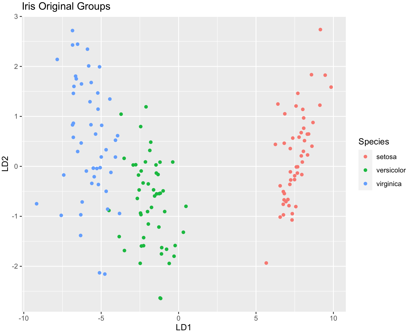
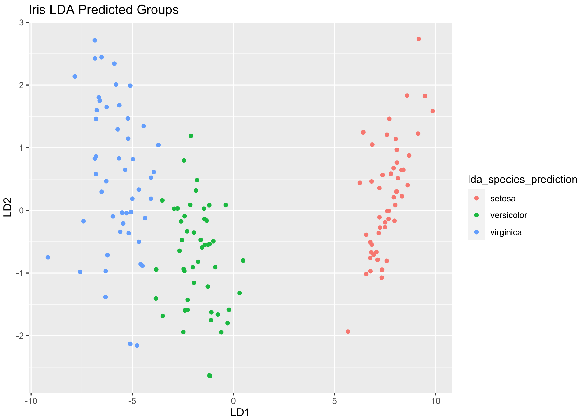
Can you find the changes on the classification between original and LDA predicted?
8.4 Cluster analysis: k-means (unsupervised)
We can use our own data without defining groups and ask if an algorithm used to find homogeneous subgroups in our data. One of such approaches is k-means clustering and we can use the preloaded function kmeans().
We will use the iris_dataset and assume that there are 3 groups (as we know about such dataset and its three putative species).
## Let's check again this dataset
iris_dataset <- iris
head(iris_dataset)
#  Sepal.Length Sepal.Width Petal.Length Petal.Width Species
#1          5.1         3.5          1.4         0.2  setosa
#2          4.9         3.0          1.4         0.2  setosa
#3          4.7         3.2          1.3         0.2  setosa
#4          4.6         3.1          1.5         0.2  setosa
#5          5.0         3.6          1.4         0.2  setosa
#6          5.4         3.9          1.7         0.4  setosa

## We need to remove the column with species assignments
iris_dataset_num <- iris_dataset[,-which(names(iris_dataset) %in% c("Species"))]
head(iris_dataset_num)
#  Sepal.Length Sepal.Width Petal.Length Petal.Width
#1          5.1         3.5          1.4         0.2
#2          4.9         3.0          1.4         0.2
#3          4.7         3.2          1.3         0.2
#4          4.6         3.1          1.5         0.2
#5          5.0         3.6          1.4         0.2
#6          5.4         3.9          1.7         0.4
Notice how I removed the “Species” column, this is one of many forms to remove columns by name. Now we determine the 3 groups with centers = 3 by repeating 30 times using the argument nstart = 30 with the function kmeans().
iris_dataset_kmeans <- kmeans(iris_dataset_num, centers = 3, nstart = 30)
iris_dataset_kmeans
#K-means clustering with 3 clusters of sizes 50, 62, 38
#
#Cluster means:
#  Sepal.Length Sepal.Width Petal.Length Petal.Width
#1     5.006000    3.428000     1.462000    0.246000
#2     5.901613    2.748387     4.393548    1.433871
#3     6.850000    3.073684     5.742105    2.071053
#
#Clustering vector:
#  [1] 1 1 1 1 1 1 1 1 1 1 1 1 1 1 1 1 1 1 1 1 1 1 1 1 1 1 1 1 1 1 1 1 1 1 1 1 1 1 1 1 1 1 1 1 1 1 1 1 1 1 2 2 3 2 2 2 2 2 2 2 2 2 2 2 2 2 2 2 2
# [70] 2 2 2 2 2 2 2 2 3 2 2 2 2 2 2 2 2 2 2 2 2 2 2 2 2 2 2 2 2 2 2 3 2 3 3 3 3 2 3 3 3 3 3 3 2 2 3 3 3 3 2 3 2 3 2 3 3 2 2 3 3 3 3 3 2 3 3 3 3
#[139] 2 3 3 3 2 3 3 3 2 3 3 2
#
#Within cluster sum of squares by cluster:
#[1] 15.15100 39.82097 23.87947
# (between_SS / total_SS =  88.4 %)
#
#Available components:
#
#[1] "cluster"      "centers"      "totss"        "withinss"     "tot.withinss" "betweenss"    "size"         "iter"         "ifault"
You can check how good the classification was based on the between_SS / total_SS value. The closer this value is to 100%, the better it is. In this case, we got 88.4%, which is very good. We can add these groupings provided by the Clustering vector that is called with iris_dataset_kmeans$cluster and add those to our dataframe and compare it those with the original species names.
## add the cluster vector to iris_dataset
iris_dataset_kmeans$cluster
# [1] 1 1 1 1 1 1 1 1 1 1 1 1 1 1 1 1 1 1 1 1 1 1 1 1 1 1 1 1 1 1 1 1 1 1 1 1 1 1 1 1 1 1 1 1 1 1 1 1 1 1 2 2 3 2 2 2 2 2 2 2 2 2 2 2 2 2 2 2 2
# [70] 2 2 2 2 2 2 2 2 3 2 2 2 2 2 2 2 2 2 2 2 2 2 2 2 2 2 2 2 2 2 2 3 2 3 3 3 3 2 3 3 3 3 3 3 2 2 3 3 3 3 2 3 2 3 2 3 3 2 2 3 3 3 3 3 2 3 3 3 3
#[139] 2 3 3 3 2 3 3 3 2 3 3 2
iris_dataset_original$kmeans_cluster <- factor(iris_dataset_kmeans$cluster)
head(iris_dataset_original)
# Species LD1 LD2 kmeans_cluster
#1 setosa 8.061800 0.3004206 1
#2 setosa 7.128688 -0.7866604 1
#3 setosa 7.489828 -0.2653845 1
#4 setosa 6.813201 -0.6706311 1
#5 setosa 8.132309 0.5144625 1
#6 setosa 7.701947 1.4617210 1
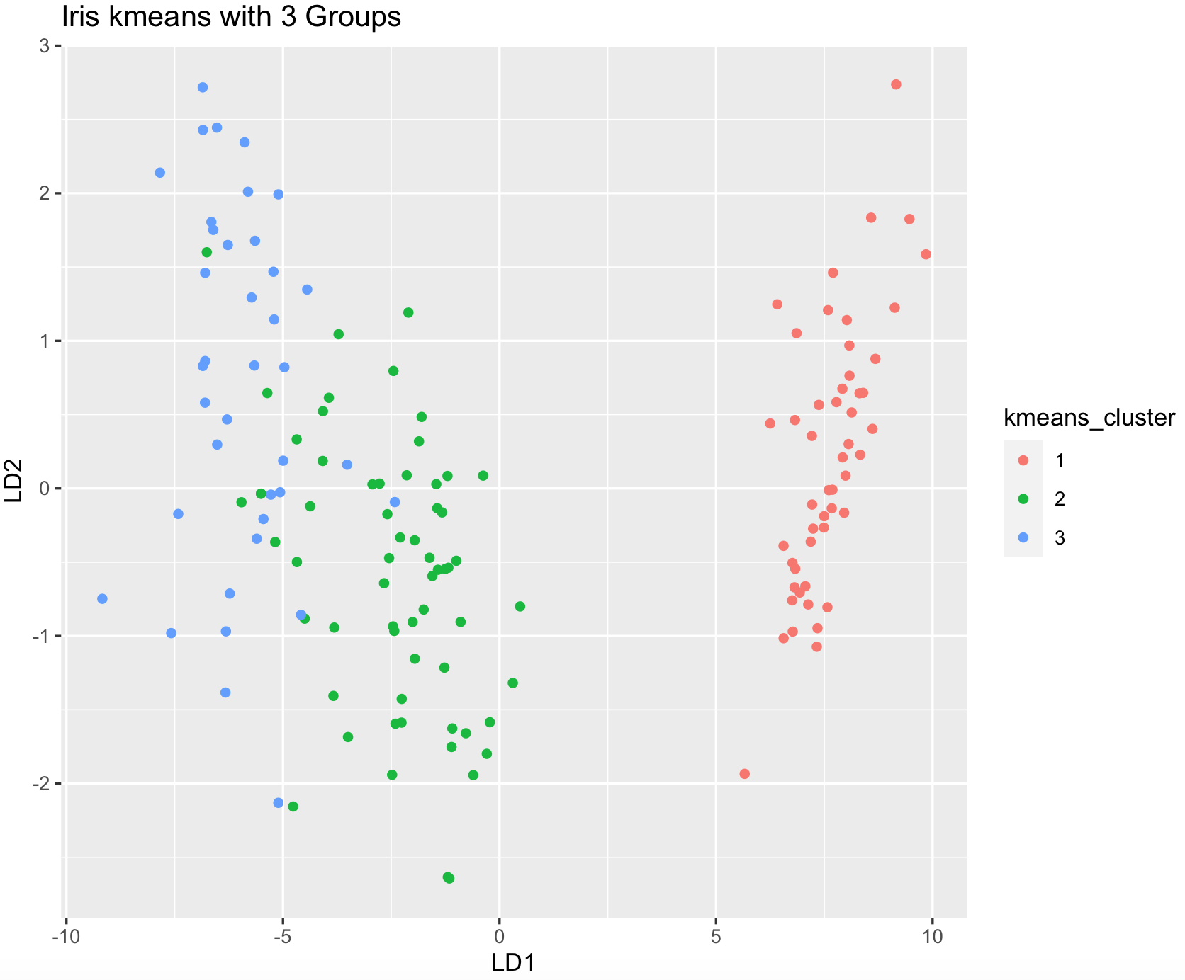
## we can plot these groups using the lda coordinates to visualize.
dev.new()
ggplot(iris_dataset_original, aes(LD1, LD2)) +
geom_point(aes(color = kmeans_cluster)) +
ggtitle("Iris kmeans with 3 Groups")