Session 5 – Getting Biological Data from Public Repositories
5.1 NCBI databases: GenBank and others
1) The NCBI (National Center for Biotechnology Information) is likely the ultimate source of public information that includes nucleotide sequences (including genomes, transcriptomes) and protein data. The NCBI goal, as is stated, is to advance science and health by providing access to biomedical and genomic information. Therefore, at some point during any your research (if that involves DNA, RNA or proteins), you will visit NCBI to retrieve or deposit molecular data. Likewise, you can access through the NCBI website an extensive literature repository named PubMed. This archive comprises more than 30 million citations for biomedical literature from MEDLINE, life science journals, and online books. Citations may include links to full-text content from PubMed Central and publisher web sites. During this class, we will focus on only few aspects of the NCBI and mostly relevant to retrieve sample data (or your own project data).
2) We can start by exploring data deposited from a poison frog Allobates kingsburyi. For this purpose, we type (or copy-and-paste) the name of this species on the search tab.

For this taxon, NCBI will return results found in several databases as indicated below.
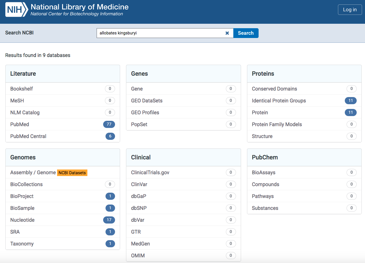
In the Literature database, it will return two links with results in the PubMed it will provide a new tab with publications that include this species. and the PubMed Central it will provide a link to the PMC database that contains 6 publications that include this species name. In the Proteins database, it will return 11 results in both the Identical Protein Groups and Protein. This is a collection amino acid sequences associated to this species name. In the Genomes database, it will return several results associated with BioProject, BioSample, Nucleotide, SRA and Taxonomy. The Nucleotide will provide link to the nuccore database that contains a collection 17 nucleotide sequences associated to this species name. Likewise, Taxonomy and it will provide link to the taxonomy database that contains the taxonomic link to the species that we are searching Allobates kingsburyi. For the Genes, Clinical, and PubChem databases, we found that they do not contain results (i.e., 0) as of February, 2025.
3) For a model system like Xenopus laevis, we will get far more results on our NCBI search. In this case, you will get an access to the genome assembly of this species (i.e., Xenopus_laevis_v10.1). Some other highlights include that this taxon has more than ~60K associated publications, gene expression omnibus (GEO) has ~190K entries, 149K protein entries, ~1.4M nucleotide entries, ~8K SRA (NGS: sequence read archive) entries, and much more. This example provides the extent of the NCBI as central and extensive archive for biological information.
4) We will explore NCBI nucleotide database to understand how the R-package rentrez can retrieve data as data frames in the R environment.
We will collect some acetylcholine receptor CHRNB2 data of frogs. For this purpose, we need to retrieve the NCBI accession numbers. Each of these is a unique identifier for a sequence record and it applies to the complete record. These ID numbers are usually a combination of a letter(s) and numbers. Versions on these accession numbers are indicated by a number after a period. For example, MF580102.1 is for the partial sequence of CHRNB2 isolated from Allobates kingsburyi and it will be the first version of this entry.
For our example taxon, we search Allobates kingsburyi on the NCBI search tab.

Next, we click on Nucleotide in the Genomes menu.
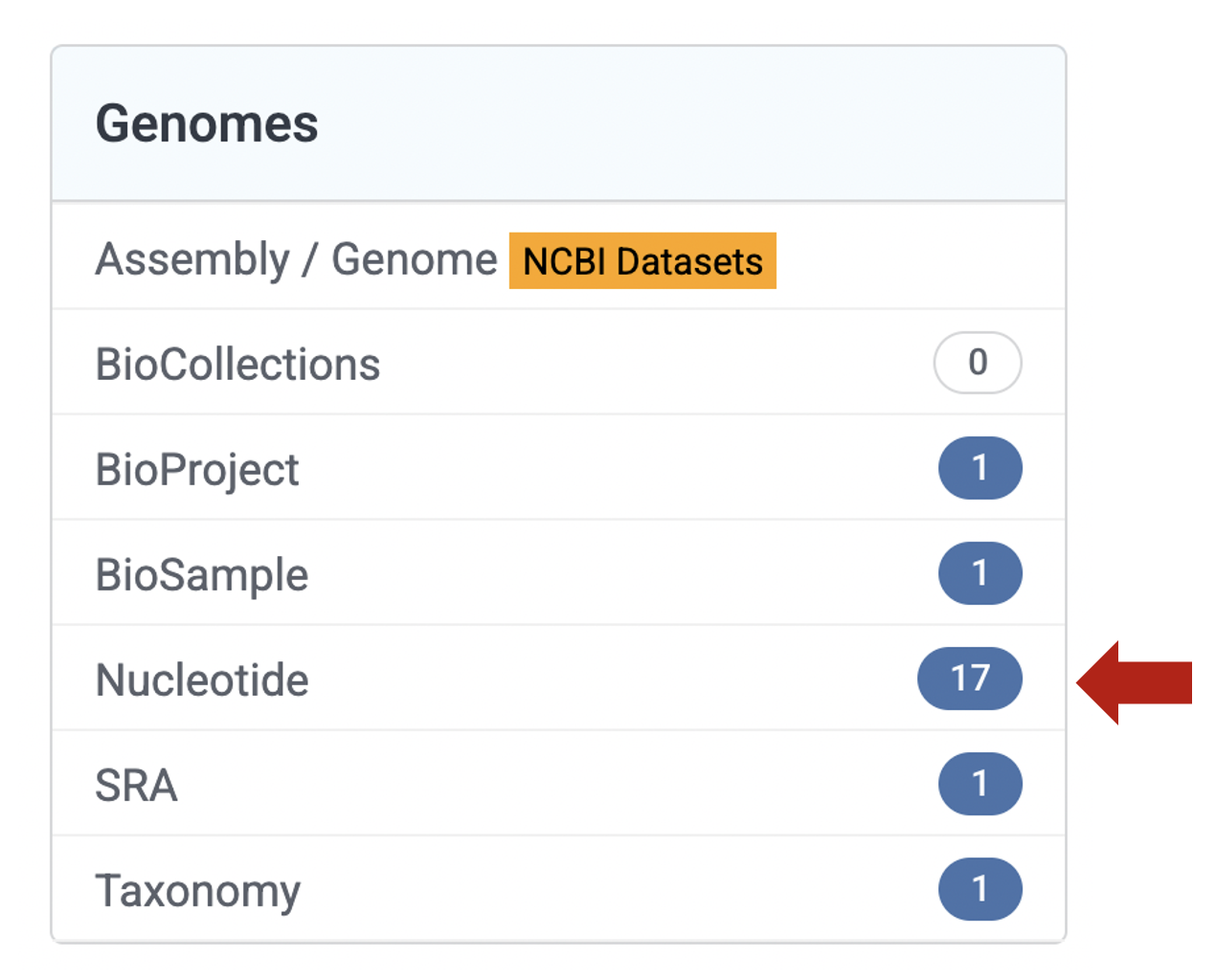
This will take us to a collection of nucleotide sequences of our target species Allobates kingsburyi. We are interested in the nicotinic acetylcholine receptor beta-2 (chrnb2) gene, partial cds.
This is is a link to the CHRNB2 sequence of Allobates kingsburyi and it will include all associated information with the accession number MF580102.1 for CHRNB2 of Allobates kingsburyi.
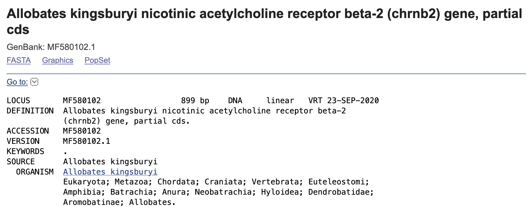
This is an extensive list and also include sequence features, gene, mRNA, CDS (coding sequence), amino acid translation, and nucleotide sequence
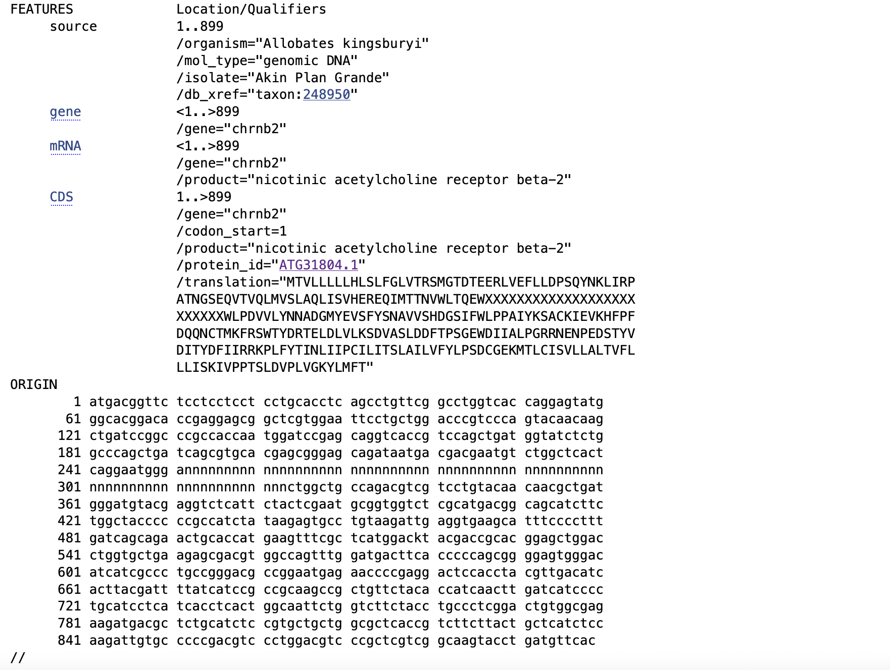
Likewise, you can get the fasta sequences of the coding section by clickling on CDS and then on the FASTA link.
You can copy and paste the output in a text file to import this later into R for further exploration.
Notice that we can obtain the same sequence in a ready to use FASTA format when we use the R-package rentrez if the accession number is known.
5.2 Accessing NCBI within R: rentrez
5) The above approach could be tedious and dependes on lots of copy-and-paste actions. However, this can be streamlined using rentrez as long as you know what accession numbers in the NCBI. rentrez has extensive vignettes here
We will proceed to get all the sequences associated to CHRNB2 in frogs by searching a set sequences of this gene. For this purpose, we start by installing (if necesseray) or load rentrez in to the R environment.
## We have downloaded this R-package before, so you just need to load it in the R environment.
library(rentrez)
## We define our working folder, where we can download our retrieved sequences -- THIS IS EXCLUSIVE FOR YOUR COMPUTER AND IT IS NOT THE PATH SHOWN BELOW
setwd("~/Desktop/Teach_R/class_pages_reference/bioinformatics_gitbook_1/my_working_directory")
Second, we can get an idea of the databases that rentrez can access from the NCBI using the EUtils API. The information about these databases can be easily accessed using the function entrez_dbs().
entrez_dbs()
#  [1] "pubmed"          "protein"         "nuccore"         "ipg"             "nucleotide"      "structure"       "genome"
# [8] "annotinfo"       "assembly"        "bioproject"      "biosample"       "blastdbinfo"     "books"           "cdd"
#[15] "clinvar"         "gap"             "gapplus"         "grasp"           "dbvar"           "gene"            "gds"
#[22] "geoprofiles"     "medgen"          "mesh"            "nlmcatalog"      "omim"            "orgtrack"        "pmc"
#[29] "proteinclusters" "pcassay"         "protfam"         "pccompound"      "pcsubstance"     "seqannot"        "snp"
#[36] "sra"
We can access at least 36 databases. We notice that this list of databases is "nuccore" is an output of entrez_dbs() which is the main repository of nucleotide sequences. Moreover, we can explore this database with three functions of rentrez: entrez_db_summary(), entrez_db_searchable() and entrez_db_links().
# Brief description of what the database is
entrez_db_summary("nuccore")
#DbName: nuccore
#MenuName: Nucleotide
#Description: Core Nucleotide db
#DbBuild: Build250217-2005m.1
#Count: 648904443
#LastUpdate: 2025/02/18 23:22

# Set of search terms that can used with this database
entrez_db_searchable("nuccore")
#Searchable fields for database 'nuccore'
#  ALL   All terms from all searchable fields
#  UID   Unique number assigned to each sequence
#  FILT      Limits the records
#  WORD      Free text associated with record
#  TITL      Words in definition line
#  KYWD      Nonstandardized terms provided by submitter
#  AUTH      Author(s) of publication
#  JOUR      Journal abbreviation of publication
#  VOL   Volume number of publication
#  ISS   Issue number of publication
#  PAGE      Page number(s) of publication
#  ORGN      Scientific and common names of organism, and all higher levels of taxonomy
#  ACCN      Accession number of sequence
#  PACC      Does not include retired secondary accessions
#  GENE      Name of gene associated with sequence
#  PROT      Name of protein associated with sequence
#  ECNO      EC number for enzyme or CAS registry number
#  PDAT      Date sequence added to GenBank
#  MDAT      Date of last update
#  SUBS      CAS chemical name or MEDLINE Substance Name
#  PROP      Classification by source qualifiers and molecule type
#  SQID      String identifier for sequence
#  GPRJ      BioProject
#  SLEN      Length of sequence
#  FKEY      Feature annotated on sequence
#  PORG      Scientific and common names of primary organism, and all higher levels of taxonomy
#  COMP      Component accessions for an assembly
#  ASSM      Assembly
#  DIV   Division
#  STRN      Strain
#  ISOL      Isolate
#  CULT      Cultivar
#  BRD   Breed
#  BIOS      BioSample

# Set of databases that might contain linked records
entrez_db_links("nuccore")
#Databases with linked records for database 'nuccore'
# [1] assembly        assembly        biocollections  bioproject      bioproject      bioproject      biosample       biosystems
# [9] ccds            clone           nuccore         dbvar           gene            genome          genome          geoprofiles
#[17] homologene      nuccore         nuccore         nuccore         nuccore         nuccore         nuccore         nuccore
#[25] nuccore         nuccore         nuccore         omim            pccompound      pcsubstance     pmc             popset
#[33] probe           protein         protein         protein         protein         protein         protein         protein
#[41] protein         proteinclusters pubmed          pubmed          pubmed          snp             sparcle         sra
#[49] sra             structure       taxonomy        trace
To download the acetylcholine receptor dataset of frogs, we kcan explore the results of a nuccore with a accession number MF580102.1 for CHRNB2 of Allobates kingsburyi.
my_MF580102 <- entrez_search(db = "nuccore", term =  "MF580102.1")
my_MF580102
#Entrez search result with 1 hits (object contains 1 IDs and no web_history object)
# Search term (as translated):
str(my_MF580102)
#List of 5
# $ ids             : chr "1248341807"
# $ count           : int 1
# $ retmax          : int 1
# $ QueryTranslation: chr ""
# $ file            :Classes 'XMLInternalDocument', 'XMLAbstractDocument' <externalptr>
# - attr(*, "class")= chr [1:2] "esearch" "list"
We can now import this sequence to R using entrez_fetch() and the results for sequence ids.
# sequence Id for Allobates kingsburyi CHRNB2
my_MF580102$ids
#[1] "1248341807"
# retrieving this sequence

my_MF580102_data <- entrez_fetch(db = "nuccore",
                                 id = my_MF580102$ids,
                            rettype = "fasta")

cat(my_MF580102_data)
#>MF580102.1 Allobates kingsburyi nicotinic acetylcholine receptor beta-2 (chrnb2) gene, partial cds
#ATGACGGTTCTCCTCCTCCTCCTGCACCTCAGCCTGTTCGGCCTGGTCACCAGGAGTATGGGCACGGACA
#CCGAGGAGCGGCTCGTGGAATTCCTGCTGGACCCGTCCCAGTACAACAAGCTGATCCGGCCCGCCACCAA
#TGGATCCGAGCAGGTCACCGTCCAGCTGATGGTATCTCTGGCCCAGCTGATCAGCGTGCACGAGCGGGAG
#CAGATAATGACGACGAATGTCTGGCTCACTCAGGAATGGGANNNNNNNNNNNNNNNNNNNNNNNNNNNNN
#NNNNNNNNNNNNNNNNNNNNNNNNNNNNNNNNNNNNNNNNNNNCTGGCTGCCAGACGTCGTCCTGTACAA
#CAACGCTGATGGGATGTACGAGGTCTCATTCTACTCGAATGCGGTGGTCTCGCATGACGGCAGCATCTTC
#TGGCTACCCCCCGCCATCTATAAGAGTGCCTGTAAGATTGAGGTGAAGCATTTCCCCTTTGATCAGCAGA
#ACTGCACCATGAAGTTTCGCTCATGGACKTACGACCGCACGGAGCTGGACCTGGTGCTGAAGAGCGACGT
#GGCCAGTTTGGATGACTTCACCCCCAGCGGGGAGTGGGACATCATCGCCCTGCCGGGACGCCGGAATGAG
#AACCCCGAGGACTCCACCTACGTTGACATCACTTACGATTTTATCATCCGCCGCAAGCCGCTGTTCTACA
#CCATCAACTTGATCATCCCCTGCATCCTCATCACCTCACTGGCAATTCTGGTCTTCTACCTGCCCTCGGA
#CTGTGGCGAGAAGATGACGCTCTGCATCTCCGTGCTGCTGGCGCTCACCGTCTTCTTACTGCTCATCTCC
#AAGATTGTGCCCCCGACGTCCCTGGACGTCCCGCTCGTCGGCAAGTACCTGATGTTCAC
We can try to retrieve related sequences of this CHRNB2 sequence using term that searches the nuccore database and retrieves all related sequences to the my_MF580102$ids (i.e., 1248341807).
To do this we use entrez_search() and add the term = "popset+representative+uid+1248341807[word]". Note that I included nuccore 1248341807 explicitly included, as shown below.
my_related_nuccore_sequences <- entrez_search(db = "nuccore", term = "popset+representative+uid+1248341807[word]")
my_related_nuccore_sequences
#Entrez search result with 0 hits (object contains 0 IDs and no web_history object)
# Search term (as translated):  (popset+representative+uid+1248341807[word])
Unfortunately, we fail to retrieve any related sequences to our sequence due to the now-retired PopSet database being no longer easily accessible. This crucial dataset was deactivated in January 2025.
This can be remediated in a more cumbersome way, but this will still allow us to retrieve related sequences.
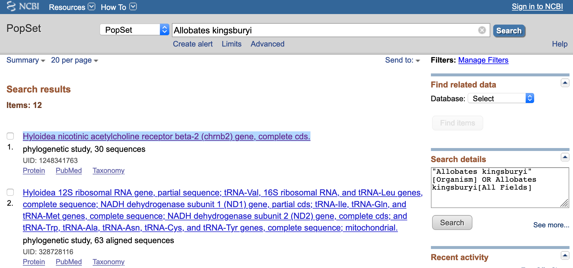
For this purpose, we need to go to the NCBI and search MF580102.1 such as we did in the previous section.
Then click on PopSet Members
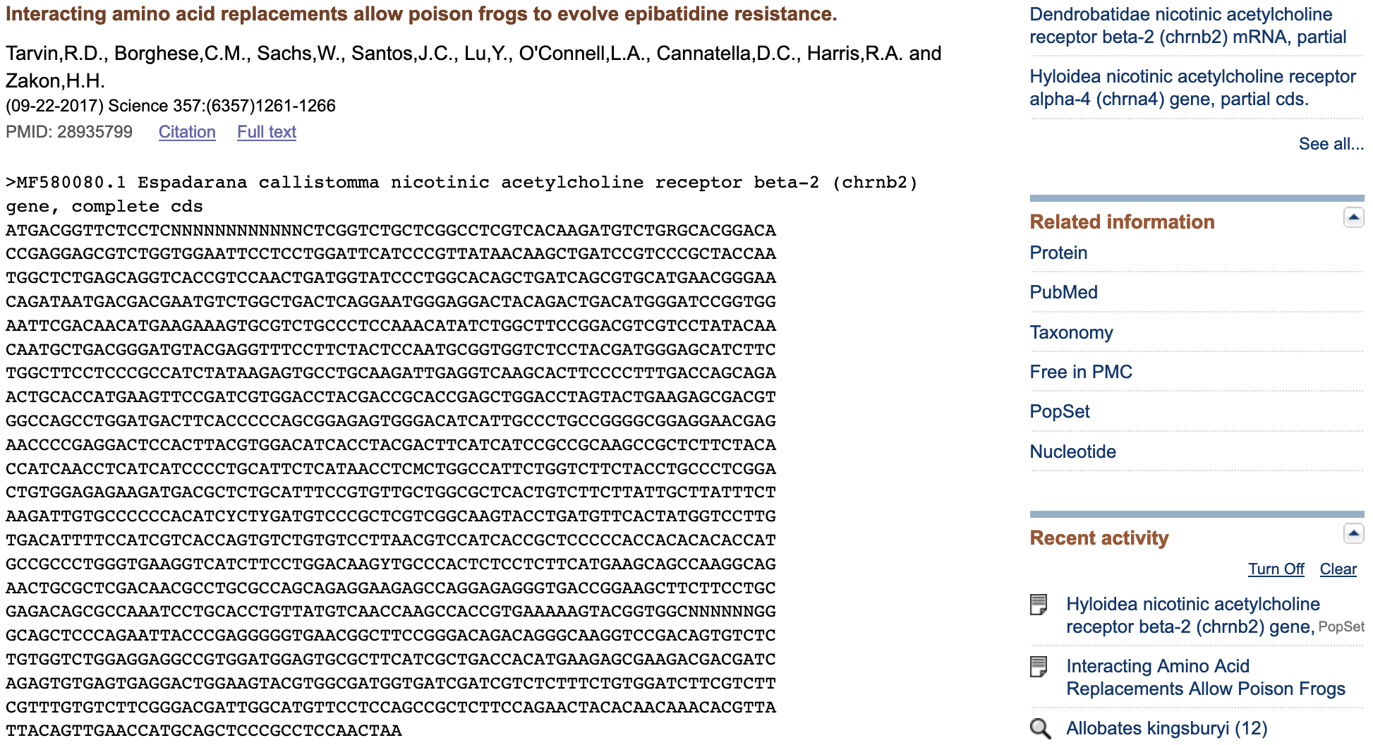
In the resulting link, a key piece of information will be displayed such to indicate were to donwload related sequences for CHRNB2 of frogs.

With this number (1248341763), we can use rentrez to find related sequences to our CHRNB2 of Allobates kingsburyi. To do this, we need to provide a term that searches the nuccore database and retrieves all related sequences by using popset+representative+uid+1248341763[word].
my_related_nuccore_sequences <- entrez_search(db = "nuccore", term = "popset+representative+uid+1248341763[word]")
my_related_nuccore_sequences
#Entrez search result with 30 hits (object contains 20 IDs and no web_history object)
# Search term (as translated):  popset+representative+uid+1248341763[word]
str(my_related_nuccore_sequences)
#List of 5
# $ ids             : chr [1:20] "1248341821" "1248341819" "1248341817" "1248341815" ...
# $ count           : int 30
# $ retmax          : int 20
# $ QueryTranslation: chr "popset+representative+uid+1248341763[word]"
# $ file            :Classes 'XMLInternalDocument', 'XMLAbstractDocument' <externalptr>
# - attr(*, "class")= chr [1:2] "esearch" "list"
my_related_nuccore_sequences_ids <- my_related_nuccore_sequences$ids
my_related_nuccore_sequences_ids
# [1] "1248341821" "1248341819" "1248341817" "1248341815" "1248341813" "1248341811" "1248341809" "1248341807" "1248341805" "1248341803"
#[11] "1248341801" "1248341799" "1248341797" "1248341795" "1248341793" "1248341791" "1248341789" "1248341787" "1248341785" "1248341783"

# we need to append the original nuccore `1248341763`
my_related_nuccore_sequences_ids <- c(1248341763, my_related_nuccore_sequences_ids)
my_related_nuccore_sequences_ids
# [1] "1248341763" "1248341821" "1248341819" "1248341817" "1248341815" "1248341813" "1248341811" "1248341809" "1248341807" "1248341805"
#[11] "1248341803" "1248341801" "1248341799" "1248341797" "1248341795" "1248341793" "1248341791" "1248341789" "1248341787" "1248341785"
#[21] "1248341783"
Now, we can fecth these sequences into R using the function entrez_fetch().
acetylcholine_receptor_data <- entrez_fetch(db = "nuccore",
                                            id = my_related_nuccore_sequences_ids,
                                       rettype = "fasta")
acetylcholine_receptor_data
#[1] ">MF580080.1 Espadarana callistomma nicotinic acetylcholine receptor beta-2 (chrnb2) gene, complete cds\nATGACGGTTCTCCTC..."
Finally, we can save them in a character vector and into a text file as we did before using the function write().
name_of_file <- paste0("acetylcholine_receptor_nuccore_data.txt")
name_of_file
#[1] "acetylcholine_receptor_nuccore_data.txt"
write(acetylcholine_receptor_data, file = name_of_file)
6) It is important to reiterate that rentrez can get us more information associated to our focal dataset of CHRNB2 of frogs with id 1248341763. Here are some interesting explorations on this accession number.
We can get the associated data link to the nuccore 1248341763. Using the function entrez_link()
my_nuccore_links <- entrez_link(dbfrom='nuccore', id=1248341763, db='all')
str(my_nuccore_links)
#List of 2
# $ links:List of 5
#  ..$ nuccore_popset  : chr "1248341763"
#  ..$ nuccore_protein : chr "1248341764"
#  ..$ nuccore_pubmed  : chr "28935799"
#  ..$ nuccore_taxonomy: chr "526126"
#  ..$ nuccore_pmc     : chr "5834227"
#  ..- attr(*, "class")= chr [1:2] "elink_classic" "list"
# $ file :Classes 'XMLInternalElementNode', 'XMLInternalNode', 'XMLAbstractNode' <externalptr>
# - attr(*, "content")= chr " $links: IDs for linked records from NCBI\n "
# - attr(*, "class")= chr [1:2] "elink" "list"
We see that the literature database nuccore_pmc has one entry and this is likely the publication associated with nuccore 1248341763. We can retrieve this information with the function entrez_fetch(). In this case, we will use a complex notation to retrieve a pmc dataset as my_nuccore_links$links$nuccore_pmc. This indicates that with the list named my_nuccore_links, we want to retrieve the list named links and the element named nuccore_pmc. When ready, we will use the function entrez_fetch() with the return format as rettype="native".
my_nuccore_links$links$nuccore_pmc
#[1] "5834227"
pmc_ids <- my_nuccore_links$links$nuccore_pmc
pmc_ids
#[1] "5834227"
my_literature <- entrez_fetch(db = "pmc", id = pmc_ids, rettype="native")
my_literature
#[1] "1:  Interacting Amino Acid Replacements Allow Poison Frogs to Evolve Epibatidine Resistance\nRebecca D. Tarvin, Cecilia M. Borghese, Wiebke Sachs, Juan C. Santos, Ying Lu, Lauren A. O’Connell, David C. Cannatella, R. Adron Harris, Harold H. Zakon\nScience. Author manuscript; available in PMC 2018 Mar 22.Published in final edited form as: Science. 2017 Sep 22; 357(6357): 1261–1266.  doi: 10.1126/science.aan5061\nPMCID: PMC5834227\n\n"
cat(my_literature)
#1:  Interacting Amino Acid Replacements Allow Poison Frogs to Evolve Epibatidine Resistance
#Rebecca D. Tarvin, Cecilia M. Borghese, Wiebke Sachs, Juan C. Santos, Ying Lu, Lauren A. O’Connell, David C. Cannatella, R. Adron Harris, Harold H. Zakon
#Science. Author manuscript; available in PMC 2018 Mar 22.Published in final edited form as: Science. 2017 Sep 22; 357(6357): 1261–1266.  doi: 10.1126/science.aan5061
#PMCID: PMC5834227
We can also retrieve the amino acid sequence associated with nuccore 1248341763 and other related protein sequences. It is very important that you use this nuccore number 1248341763 to retrieve related protein sequences in the term input as popset+representative+uid+1248341763[word].
my_nuccore_links$links$nuccore_protein
#[1] "1248341764"
protein_ids <- my_nuccore_links$links$nuccore_protein
protein_ids
#[1] "1248341764"
my_related_protein_sequences <- entrez_search(db = "protein", term = "popset+representative+uid+1248341763[word]")
my_related_protein_sequences
#Entrez search result with 30 hits (object contains 20 IDs and no web_history object)
# Search term (as translated):  popset+representative+uid+1248341763[word]
str(my_related_protein_sequences)
#List of 5
# $ ids             : chr [1:20] "1248341822" "1248341820" "1248341818" "1248341816" ...
# $ count           : int 30
# $ retmax          : int 20
# $ QueryTranslation: chr "popset+representative+uid+1248341763[word]"
# $ file            :Classes 'XMLInternalDocument', 'XMLAbstractDocument' <externalptr>
# - attr(*, "class")= chr [1:2] "esearch" "list"
my_related_protein_sequences_ids <- my_related_protein_sequences$ids
my_related_protein_sequences_ids
# [1] "1248341822" "1248341820" "1248341818" "1248341816" "1248341814" "1248341812" "1248341810" "1248341808" "1248341806" "1248341804"
#[11] "1248341802" "1248341800" "1248341798" "1248341796" "1248341794" "1248341792" "1248341790" "1248341788" "1248341786" "1248341784"

# we need to append the original PROTEIN "1248341764"

my_related_protein_sequences_ids <- c(1248341764, my_related_protein_sequences_ids)
my_related_protein_sequences_ids
# [1] "1248341764" "1248341822" "1248341820" "1248341818" "1248341816" "1248341814" "1248341812" "1248341810" "1248341808" "1248341806"
#[11] "1248341804" "1248341802" "1248341800" "1248341798" "1248341796" "1248341794" "1248341792" "1248341790" "1248341788" "1248341786"
#[21] "1248341784"
Now, we can retrive and save these data in a text file using fasta format.
acetylcholine_receptor_protein_data <- entrez_fetch(db = "protein", id = my_related_protein_sequences_ids, rettype="fasta")
acetylcholine_receptor_protein_data

#[1] ">ATG31782.1 nicotinic acetylcholine receptor beta-2 [Espadarana callistomma]\nMTVLLXXXXLGLLGLVTRCLXTDTEERLVEFLLDSSRYNKLIRPA...

cat(acetylcholine_receptor_protein_data)

#>ATG31782.1 nicotinic acetylcholine receptor beta-2 [Espadarana callistomma]
#MTVLLXXXXLGLLGLVTRCLXTDTEERLVEFLLDSSRYNKLIRPATNGSEQVTVQLMVSLAQLISVHERE
#QIMTTNVWLTQEWEDYRLTWDPVEFDNMKKVRLPSKHIWLPDVVLYNNADGMYEVSFYSNAVVSYDGSIF
#WLPPAIYKSACKIEVKHFPFDQQNCTMKFRSWTYDRTELDLVLKSDVASLDDFTPSGEWDIIALPGRRNE
#NPEDSTYVDITYDFIIRRKPLFYTINLIIPCILITSLAILVFYLPSDCGEKMTLCISVLLALTVFLLLIS
#KIVPPTSLDVPLVGKYLMFTMVLVTFSIVTSVCVLNVHHRSPTTHTMPPWVKVIFLDKLPTLLFMKQPRQ
#NCARQRLRQQRKSQERVTGSFFLRDSAKSCTCYVNQATVKKYGGXXGQLPELPEGVNGFRDRQGKVRQCL
#CGLEEAVDGVRFIADHMKSEDDDQSVSEDWKYVAMVIDRLFLWIFVFVCVFGTIGMFLQPLFQNYTTNTL
#LQLNHAAPASN

name_of_file <- paste0("acetylcholine_receptor_protein_data.txt")
name_of_file
#[1] "acetylcholine_receptor_protein_data.txt"
write(acetylcholine_receptor_protein_data, file = name_of_file)
7) To import these data back to R , we need the path to the files that contain the data using the R-package Biostrings.
We can import the nucleotide sequences as DNAstrings.
## you might have already installed the library Biostrings
library(Biostrings)
## get the path to the file with the nucleotide sequences -- THIS IS EXCLUSIVE FOR YOUR COMPUTER AND IT IS NOT THE PATH SHOWN BELOW
my_nuccore_as_dna_stringset <- readDNAStringSet(filepath = "~/Desktop/Teach_R/class_pages_reference/bioinformatics_gitbook_1/my_working_directory/acetylcholine_receptor_nuccore_data.txt",
                                         format = "fasta")
my_nuccore_as_dna_stringset

# DNAStringSet object of length 21:
#     width seq                                                                                                                   names
# [1]  1506 ATGACGGTTCTCCTCNNNNNNNNNNNNCTCGGTCTGCTCGGCCTCGTCACAAGATGT...AACTACACAACAAACACGTTATTACAGTTGAACCATGCAGCTCCCGCCTCCAACTAA MF580080.1 Espada...
# [2]   195 GCTGATGGGATGTATGAGGTCTCCTTCTACTCTAACGCGGTGGTCTCGCACGACGGC...TGCACCATGAAGTTCCGCTCGTGGACTTATGACCGCACCGAGCTGGACCTGGTGCTG MF580109.1 Phyllo...
# [3]  1506 ATGACGGCTCTCCTCCTCGTCCTGCACCTCAGCCTGCTCGGCCTGGTCACCAGAAGT...AACTACACATCAAACACGTTAATACAGCTGAACCATGGGACCCCCGCCTCCAACTAA MF580108.1 Phyllo...
# [4]   203 GCTGATGGGATGTATGAGGTCTCCTTCTACTCTAACGCGGTGGTCTCACACGACGGC...GAAGTTCCGCTCATGGACTTATGACCGCACTGAGCTGGACCTGGTGCTGAAGAGTGA MF580107.1 Ranito...
# [5]   134 GCTGATGGGATGTACGAGGTCTCCTTCTACTCCAACGCGGTGGTCTCGCACGAYGGC...CGCCATCTATAAGAGCGCCTGTAAGATCGAGGTGAAGCACTTTCCGTTCGACCAGCA MF580106.1 Rheoba...
# ...   ... ...
#[17]  1506 ATGACGGCTCTCCTCCTCGTCCTGCACCTCAGCCTGCTGGGCCTGGTCACCAGAAGT...AACTACACATCAAACACGTTACTACAGCTAAACCATGGGGCTCCTGCCTCCAACTGA MF580094.1 Epiped...
#[18]  1462 AAGTATGGGCACGGACACCGAGGAGCGGCTCCTGGAATTCCTGCTGGACCCATCTCG...TCAAACACGTTACTACAGCTGAACCATGGGGCTCCTGCCTCCAACTGAAGGCGAACC MF580093.1 Epiped...
#[19]  1506 ATGACGGCTCTCCTCCTCGTCCTGCACCTCAGCCTGCTGGGCCTGGTCACCAGAAGT...AACTACACATCAAACACGTTACTACAGCTGAACCATGGGGCTCCTGCCTCCAACTGA MF580092.1 Epiped...
#[20]  1506 ATGACGGCTCTCCTCCTCGTCCTGCACCTCAGCCTGTTGGGCCTGGTCACCAGAAGT...AACTACACATCAAACACGTTACTACAGCTGAACCATGGGGCTCCTGCCTCCAACTGA MF580091.1 Epiped...
#[21]  1506 ATGACGGCTCTCCTCCTCGTCCTGCACCTCAGCCTGCTGGGCCTGGTCACCAGAAGT...AACTACACATCAAACACRTTACTACAGCTGAACCATGGGGCTCCTGCCTCCAACTGA MF580090.1 Epiped...
We can also import the amino acid sequences as AAstrings.
# get the path to the file with the amino acid sequences -- THIS IS EXCLUSIVE FOR YOUR COMPUTER AND IT IS NOT THE PATH SHOWN BELOW
my_protein_as_aa_stringset <- readAAStringSet(filepath = "~/Desktop/Teach_R/class_pages_reference/bioinformatics_gitbook_1/my_working_directory/acetylcholine_receptor_protein_data.txt",
                                         format = "fasta")
my_protein_as_aa_stringset
#AAStringSet object of length 21:
#     width seq                                                                                                                   names
# [1]   501 MTVLLXXXXLGLLGLVTRCLXTDTEERLVEFLLDSSRYNKLIRPATNGSEQVTVQLM...SVSEDWKYVAMVIDRLFLWIFVFVCVFGTIGMFLQPLFQNYTTNTLLQLNHAAPASN ATG31782.1 nicoti...
# [2]    65 ADGMYEVSFYSNAVVSHDGSIFWLPPAIYKSACKIEVKHFPFDQQNCTMKFRSWTYDRTELDLVL                                                     ATG31811.1 nicoti...
# [3]   501 MTALLLVLHLSLLGLVTRSMGTDTEERLVEFLLDPSRYNKLIRPATNGSEQVTVQLM...SVSEDWKYVAMVIDRLFLWIFVFVCVFGTIGMFLQPLFQNYTSNTLIQLNHGTPASN ATG31810.1 nicoti...
# [4]    67 ADGMYEVSFYSNAVVSHDGSIFWLPPAIYKSACKIEVKHFPFDQQNCTMKFRSWTYDRTELDLVLKS                                                   ATG31809.1 nicoti...
# [5]    44 ADGMYEVSFYSNAVVSHDGSIFWLPPAIYKSACKIEVKHFPFDQ                                                                          ATG31808.1 nicoti...
# ...   ... ...
#[17]   501 MTALLLVLHLSLLGLVTRSMGTDTEERLVEFLLDPSRYNKLIRPATNGSEQVTVQLM...SVSEDWKYVAMVIDRLFLWIFVFVCVFGTIGMFLQPLFQNYTSNTLLQLNHGAPASN ATG31796.1 nicoti...
#[18]   483 SMGTDTEERLLEFLLDPSRYNKLIRPATNGSEQVTVQLMVSLAQLISVHERXXXXXX...SVSEDWKYVAMVIDRLFLWIFVFVCVFGTIGMFLQPLFQNYTSNTLLQLNHGAPASN ATG31795.1 nicoti...
#[19]   501 MTALLLVLHLSLLGLVTRSMGTDTEERLVEFLLDPSRYNKLIRPATNGSEQVTVQLM...SVSEDWKYVAMVIDRLFLWIFVFVCVFGTIGMFLQPLFQNYTSNTLLQLNHGAPASN ATG31794.1 nicoti...
#[20]   501 MTALLLVLHLSLLGLVTRSMGTDTEERLVEFLLDPSRYNKLIRPATNGSEQVTVQLM...SVSEDWKYVAMVIDRLFLWIFVFVCVFGTIGMFLQPLFQNYTSNTLLQLNHGAPASN ATG31793.1 nicoti...
#[21]   501 MTALLLVLHLSLLGLVTRSMGTDTEERLVEFLLDPSRYNKLIRPATNGSEQVTVQLM...SVSEDWKYVAMVIDRLFLWIFVFVCVFGTIGMFLQPLFQNYTSNTLLQLNHGAPASN ATG31792.1 nicoti...
5.3 Retrieving PubMed references
We can use rentrez to retrive publication infomration relevant to a term (i.e., text argument) that you can use for citations or references. The main source of such information is PubMed and it claims to include >30 million citations for biomedical literature from MEDLINE, life science journals, and online books. Likewise, such citations may include links to full text content from PubMed Central and publisher web sites. However, from R, you will be able to access the citation, abstract and other identifiers that you can use later on PubMed website.
8) we can use publications relevant to a term of interest, for example, an genus of frogs Ameerega using the following procedure.
We can retrieve the results in the Medline format as follows.
## make sure that 'rentrez' is loaded
require(rentrez)
## retrieve IDs from NCBI
genus_publications_IDs <- entrez_search(db="pubmed", term="Ameerega")
str(genus_publications_IDs)
#List of 5
# $ ids             : chr [1:20] "39646486" "39473883" "37889647" "35391365" ...
# $ count           : int 21
# $ retmax          : int 20
# $ QueryTranslation: chr "\"Ameerega\"[All Fields]"
# $ file            :Classes 'XMLInternalDocument', 'XMLAbstractDocument' <externalptr>
# - attr(*, "class")= chr [1:2] "esearch" "list"

genus_publications_medline <- entrez_fetch(db="pubmed", id=genus_publications_IDs$ids, rettype="medline")
cat(genus_publications_medline)

#PMID- 39473883
#OWN - NLM
#STAT- PubMed-not-MEDLINE
#LR  - 20241030
#IS  - 1045-2249 (Print)
#IS  - 1465-7279 (Electronic)
#IS  - 1045-2249 (Linking)
#VI  - 35
#IP  - 6
#DP  - 2024 Nov-Dec
#TI  - Detectability of a poison frog and its Batesian mimic depends on body posture and
#      viewing angle.
#PG  - arae077
#LID - 10.1093/beheco/arae077 [doi]
#LID - arae077
#AB  - Aposematic signals warn predators that prey should be avoided due to dangerous
#      secondary defences. However, as warning signals do not always produce avoidance,
#      warning colors may evolve as a trade-off balancing detectability against signal
#      saliency. For Batesian mimics, which display salient signals but lack secondary
#      defenses, the costs of predator encounters are greater, potentially increasing
#      the benefit of crypsis. This raises the question of whether imperfect mimicry may
#      reduce detectability while retaining mimetic efficacy. We tested this hypothesis
#      with the poisonous frog Ameerega bilinguis and undefended Batesian mimic
#      Allobates zaparo, using computational visual modeling and screen-based detection
#      trials with human participants. We found that both species incorporate camouflage
#      into their warning colors, but to different degrees depending on viewing angle
#      and behavior. Contrary to expectation, we found differences in detectability
#      between model and mimic that do not adhere to the hypothesized cryptic mimetic
#      phenotype. To aerial observers, we found the mimic to be more detectable than the
#      model. To terrestrial observers, likely owing to the model's bright ventral
#      color, we found the model more detectable in viewing angles that highlight the
#      ventral coloration, whereas the mimic was more detectable in viewing angles that
#      highlight the dorsal coloration. Consequently, we suggest that in addition to
#      being the result of perceptual or developmental constraints, imperfect mimicry
#      may also evolve as an adaptive strategy which balances camouflage with different
#      signaling functions. Our findings complement the emerging view that aposematic
#      signals may evolve in response to a multitude of selection pressures beyond
#      aversion alone.
#CI  - (c) The Author(s) 2024. Published by Oxford University Press on behalf of the
#      International Society for Behavioral Ecology.
#FAU - McEwen, Brendan L
#AU  - McEwen BL
#AUID- ORCID: 0000-0003-1672-0638
#AD  - Department of Psychology, Neuroscience, & Behaviour, McMaster University,
#      Hamilton, ON L8S 4L8, Canada.
#FAU - Yeager, Justin
#AU  - Yeager J
#AUID- ORCID: 0000-0001-8692-6311
#AD  - Grupo de Investigacion en Biodiversidad, Medio Ambiente y Salud (BIOMAS),
#      Facultad de Ingenierias y Ciencas Aplicadas, Universidad de Las Americas,
#      Ecuador.
#FAU - Kinley, Isaac
#AU  - Kinley I
#AUID- ORCID: 0000-0003-2057-9606
#AD  - Department of Psychology, Neuroscience, & Behaviour, McMaster University,
#      Hamilton, ON L8S 4L8, Canada.
#AD  - Rotman Research Institute at Baycrest, Toronto, ON M6A 1W1, Canada.
#FAU - Anderson, Hannah M
#AU  - Anderson HM
#AUID- ORCID: 0000-0002-3620-4641
#AD  - Department of Psychology, Neuroscience, & Behaviour, McMaster University,
#      Hamilton, ON L8S 4L8, Canada.
#FAU - Barnett, James B
#AU  - Barnett JB
#AUID- ORCID: 0000-0001-9789-4132
#AD  - Department of Psychology, Neuroscience, & Behaviour, McMaster University,
#      Hamilton, ON L8S 4L8, Canada.
#AD  - School of Natural Sciences, Trinity College Dublin, Dublin 2 D02 PN40, Ireland.
#LA  - eng
#SI  - Dryad/10.5061/dryad.bzkh189k7
#PT  - Journal Article
#DEP - 20241004
#PL  - United States
#TA  - Behav Ecol
#JT  - Behavioral ecology : official journal of the International Society for Behavioral
#      Ecology
#JID - 9426330
#PMC - PMC11520748
#OTO - NOTNLM
#OT  - Aposematism
#OT  - Batesian mimicry
#OT  - detectability
#OT  - imperfect mimicry
#OT  - poison frogs
#OT  - visual ecology
#COIS- The authors declare they have no conflicts of interest.
#EDAT- 2024/10/30 10:54
#MHDA- 2024/10/30 10:55
#PMCR- 2024/10/04
#CRDT- 2024/10/30 04:41
#PHST- 2023/12/06 00:00 [received]
#PHST- 2024/07/17 00:00 [revised]
#PHST- 2024/10/01 00:00 [accepted]
#PHST- 2024/10/30 10:55 [medline]
#PHST- 2024/10/30 10:54 [pubmed]
#PHST- 2024/10/30 04:41 [entrez]
#PHST- 2024/10/04 00:00 [pmc-release]
#AID - arae077 [pii]
#AID - 10.1093/beheco/arae077 [doi]
#PST - epublish
#SO  - Behav Ecol. 2024 Oct 4;35(6):arae077. doi: 10.1093/beheco/arae077. eCollection
#      2024 Nov-Dec.
#...
We can save these publication refereces into a text file in your working directory.
# this is exclusive to your OWN COMPUTER change it accordingly
setwd("~/Desktop/Teach_R/my_working_directory")
write(genus_publications_medline, "my_genus_publications_as_medline_format.txt")
We can retrieve the results in the abstract format as follows.
## make sure that 'rentrez' is loaded
require(rentrez)
## retrieve IDs from NCBI
genus_publications_IDs <- entrez_search(db="pubmed", term="Ameerega")
str(genus_publications_IDs)
#List of 5
# $ ids             : chr [1:20] "39646486" "39473883" "37889647" "35391365" ...
# $ count           : int 21
# $ retmax          : int 20
# $ QueryTranslation: chr "\"Ameerega\"[All Fields]"
# $ file            :Classes 'XMLInternalDocument', 'XMLAbstractDocument' <externalptr>
# - attr(*, "class")= chr [1:2] "esearch" "list"

genus_publications_abstract <- entrez_fetch(db="pubmed", id=genus_publications_IDs$ids, rettype="abstract")
cat(genus_publications_abstract)


#Behav Ecol. 2024 Oct 4;35(6):arae077. doi: 10.1093/beheco/arae077. eCollection
#2024 Nov-Dec.
#
#Detectability of a poison frog and its Batesian mimic depends on body posture
#and viewing angle.
#
#McEwen BL(1), Yeager J(2), Kinley I(1)(3), Anderson HM(1), Barnett JB(1)(4).
#
#Author information:
#(1)Department of Psychology, Neuroscience, & Behaviour, McMaster University,
#Hamilton, ON L8S 4L8, Canada.
#(2)Grupo de Investigación en Biodiversidad, Medio Ambiente y Salud (BIOMAS),
#Facultad de Ingenierías y Ciencas Aplicadas, Universidad de Las Américas,
#Ecuador.
#(3)Rotman Research Institute at Baycrest, Toronto, ON M6A 1W1, Canada.
#(4)School of Natural Sciences, Trinity College Dublin, Dublin 2 D02 PN40,
#Ireland.
#
#Aposematic signals warn predators that prey should be avoided due to dangerous
#secondary defences. However, as warning signals do not always produce avoidance,
#warning colors may evolve as a trade-off balancing detectability against signal
#saliency. For Batesian mimics, which display salient signals but lack secondary
#defenses, the costs of predator encounters are greater, potentially increasing
#the benefit of crypsis. This raises the question of whether imperfect mimicry
#may reduce detectability while retaining mimetic efficacy. We tested this
#hypothesis with the poisonous frog Ameerega bilinguis and undefended Batesian
#mimic Allobates zaparo, using computational visual modeling and screen-based
#detection trials with human participants. We found that both species incorporate
#camouflage into their warning colors, but to different degrees depending on
#viewing angle and behavior. Contrary to expectation, we found differences in
#detectability between model and mimic that do not adhere to the hypothesized
#cryptic mimetic phenotype. To aerial observers, we found the mimic to be more
#detectable than the model. To terrestrial observers, likely owing to the model's
#bright ventral color, we found the model more detectable in viewing angles that
#highlight the ventral coloration, whereas the mimic was more detectable in
#viewing angles that highlight the dorsal coloration. Consequently, we suggest
#that in addition to being the result of perceptual or developmental constraints,
#imperfect mimicry may also evolve as an adaptive strategy which balances
#camouflage with different signaling functions. Our findings complement the
#emerging view that aposematic signals may evolve in response to a multitude of
#selection pressures beyond aversion alone.
#
#© The Author(s) 2024. Published by Oxford University Press on behalf of the
#International Society for Behavioral Ecology.
#
#DOI: 10.1093/beheco/arae077
#PMCID: PMC11520748
#PMID: 39473883
#
#Conflict of interest statement: The authors declare they have no conflicts of
#interest.
#...
We can save these publication refereces into a text file in your working directory.
# this is exclusive to your OWN COMPUTER change it accordingly
setwd("~/Desktop/Teach_R/my_working_directory")
write(genus_publications_abstract, "my_genus_publications_as_abstract_format.txt")
5.4 Comparing sequences: BLAST
One of the most important tools of the NCBI is the Basic Local Alignment Search Tool (BLAST). This tool finds regions of local similarity between sequences by comparing nucleotide or protein sequences to sequence databases and calculates the statistical significance of matches. BLAST can be accessed form the NCBI website or link provided. It also has a friendly guide.
Here is a table from the reference manual that provide you with key features of the BLAST search pages in the “Basic BLAST” category guide.
| Search page | Query & database | Alignment | Programs & Description |
|---|---|---|---|
| nucleotide blast | nucleotide vs nucleotide | nucleotide | megablast: for sequence identification, intra-species comparison, discontiguous megablast: for cross-species comparison, searching with coding sequences; blastn: for searching with shorter queries, cross-species comparison |
| protein blast | protein vs protein | protein | blastp: general sequence identification and similarity searches; Quick BLASTP: with a kmer match to accelerate search speed for very similar proteins; DELTA-BLAST[3]: protein similarity search with higher sensitivity than blastp; PSI-BLAST: iterative search for position-specific score matrix (PSSM) to identify distant relatives for a protein family; PHI-BLAST: protein alignment with input pattern as anchor_constraint |
| blastx | nucleotide (translated) vs protein | protein | blastx: for identifying potential protein products encoded by a nucleotide query |
| tblastn | protein vs nucleotide (translated) | protein | tblastn: for identifying database sequences encoding proteins similar to the query |
| tblastx | nucleotide (translated) vs nucleotide (translated) | protein | tblastx: for identifying nucleotide sequences similar to the query based on their coding potential |
We will focus on nucleotide blast.
9) If you are interested in comparing a nucleotide query against the nucleotide reference collection. You can use blastn or standard nucleotide BLAST.
For a simple query, you usually start by copying and pasting the nucleotide sequence that you want to BLAST. We will use a short sequence of the MF580102.1 NCBI accession number of the nicotinic acetylcholine receptor beta-2 (chrnb2) from Allobates kingsburyi.
>MF580102.1 Allobates kingsburyi nicotinic acetylcholine receptor beta-2 (chrnb2) gene, partial cds
ATGACGGTTCTCCTCCTCCTCCTGCACCTCAGCCTGTTCGGCCTGGTCACCAGGAGTATGGGCACGGACA
CCGAGGAGCGGCTCGTGGAATTCCTGCTGGACCCGTCCCAGTACAACAAGCTGATCCGGCCCGCCACCAA
TGGATCCGAGCAGGTCACCGTCCAGCTGATGGTATCTCTGGCCCAGCTGATCAGCGTGCACGAGCGGGAG
CAGATAATGACGACGAATGTCTGGCTCACTCAGGAATGGGANNNNNNNNNNNNNNNNNNNNNNNNNNNNN
NNNNNNNNNNNNNNNNNNNNNNNNNNNNNNNNNNNNNNNNNNNCTGGCTGCCAGACGTCGTCCTGTACAA
CAACGCTGATGGGATGTACGAGGTCTCATTCTACTCGAATGCGGTGGTCTCGCATGACGGCAGCATCTTC
TGGCTACCCCCCGCCATCTATAAGAGTGCCTGTAAGATTGAGGTGAAGCATTTCCCCTTTGATCAGCAGA
ACTGCACCATGAAGTTTCGCTCATGGACKTACGACCGCACGGAGCTGGACCTGGTGCTGAAGAGCGACGT
GGCCAGTTTGGATGACTTCACCCCCAGCGGGGAGTGGGACATCATCGCCCTGCCGGGACGCCGGAATGAG
AACCCCGAGGACTCCACCTACGTTGACATCACTTACGATTTTATCATCCGCCGCAAGCCGCTGTTCTACA
CCATCAACTTGATCATCCCCTGCATCCTCATCACCTCACTGGCAATTCTGGTCTTCTACCTGCCCTCGGA
CTGTGGCGAGAAGATGACGCTCTGCATCTCCGTGCTGCTGGCGCTCACCGTCTTCTTACTGCTCATCTCC
AAGATTGTGCCCCCGACGTCCCTGGACGTCCCGCTCGTCGGCAAGTACCTGATGTTCAC
Notice that you can paste multiple sequences in fasta format.
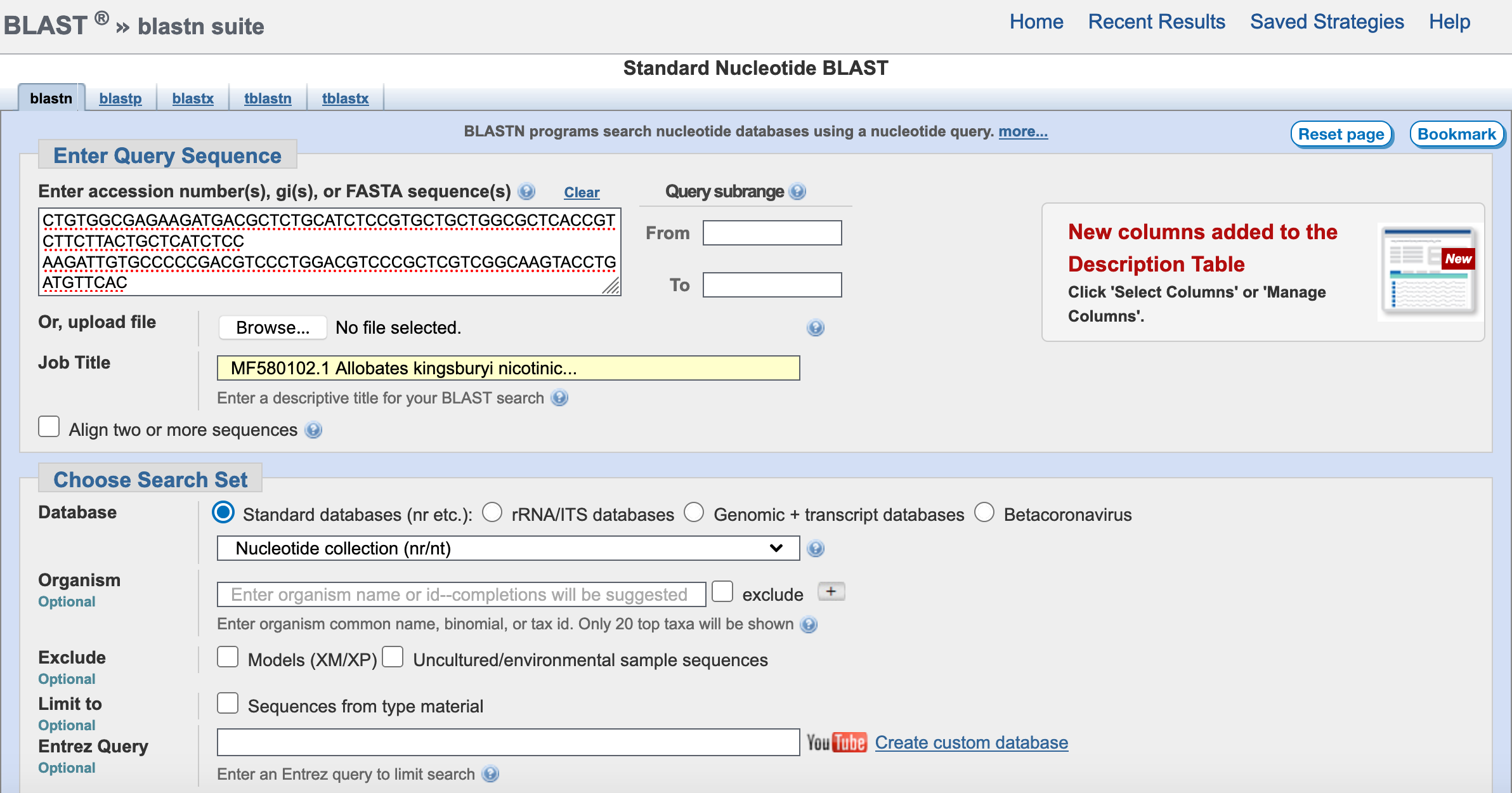
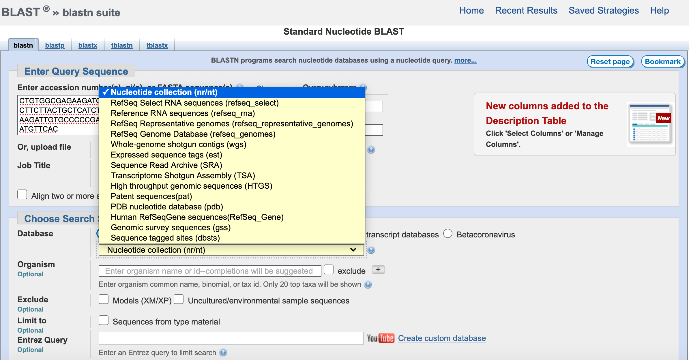
10) You have several options under Choose Search Set.
The first set is to choose a database and the default is Core nucleotide database (core_nt). However, you have other 17 databases to choose. In most cases, this database is the best option. However, the others are useful if looking in reference collections (e.g., refseq_select, refseq_rna, refseq_representative_genomes, etc.) Other dataset are more ameneable for genomic/transcriptomic datasets (e.g., wgs, SRA, TSA) and in most cases they lack annotation (i.e., gene soruce is unknown).
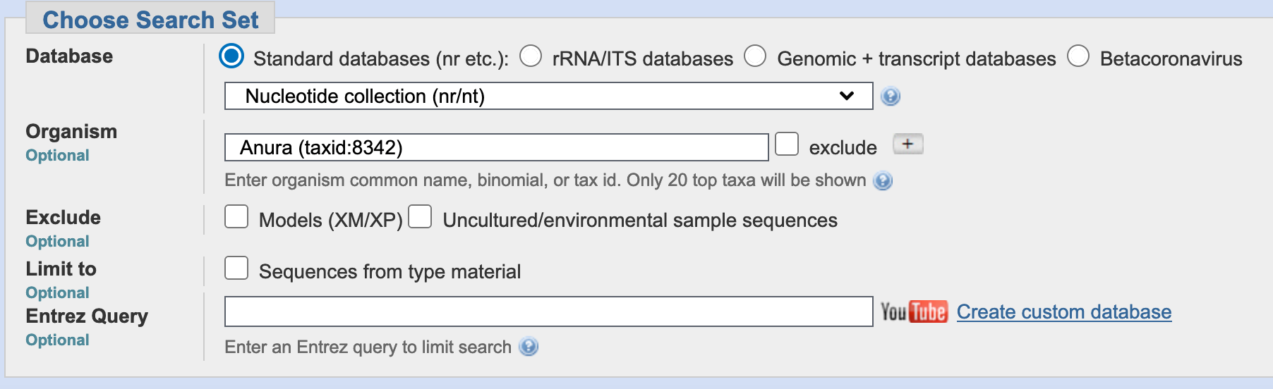
 Next, you can select the organism taxonomic level that you want to restrict you search. If left blank, it will search all taxonomic groups in that database. The lower the taxonomic level (e.g., genus versus family), the less sequences to compare the faster the BLAST will run. In this example, we will select the order Anura (all frogs.)
In the program selection, the default is highly similar sequences (megablast). This is the strictest, this approach is intended for comparing a query to closely related sequences and works best if the target percent identity is 95% or more but is very fast. The option somewhat similar sequences (blastn) is slow but allows a word-size down to seven bases (you can recover more matches). Likewise, you can modify the General Parameters from its default values. In most cases before running BLAST, you leave them in their default. For our example, we will select blastn with other parameters in default.
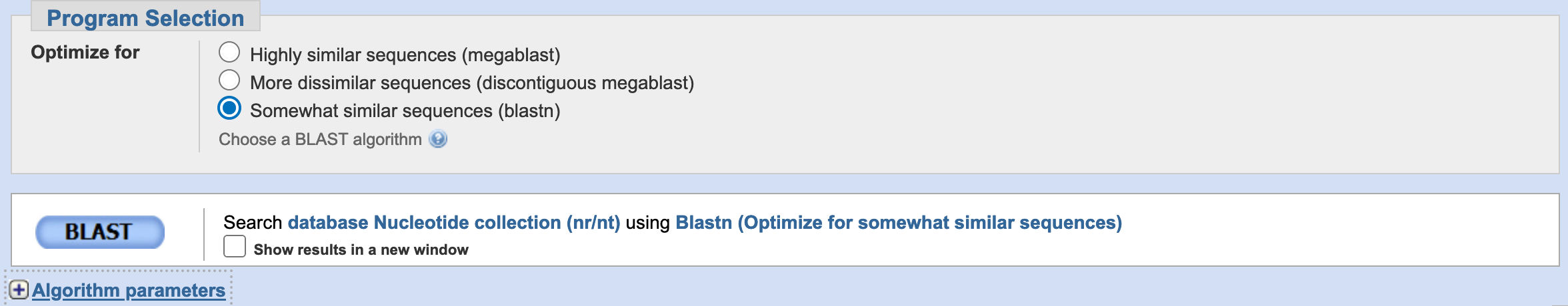
Then, we click BLAST.
11) After you submit your query, you might need to wait for seconds to minutes. This time is not consistent and it depends on the NCBI servers as well as “fair time use”. This refers to using the NCBI searches system responsibly to prevent overloading it with excessively large or frequent queries. This ensures that all users can access the tool efficiently. It includes limitations on sequence length per search and guidelines on search frequency to prevent exceeding allocated CPU time, promoting equitable access for everyone.
Here is the output of our search.
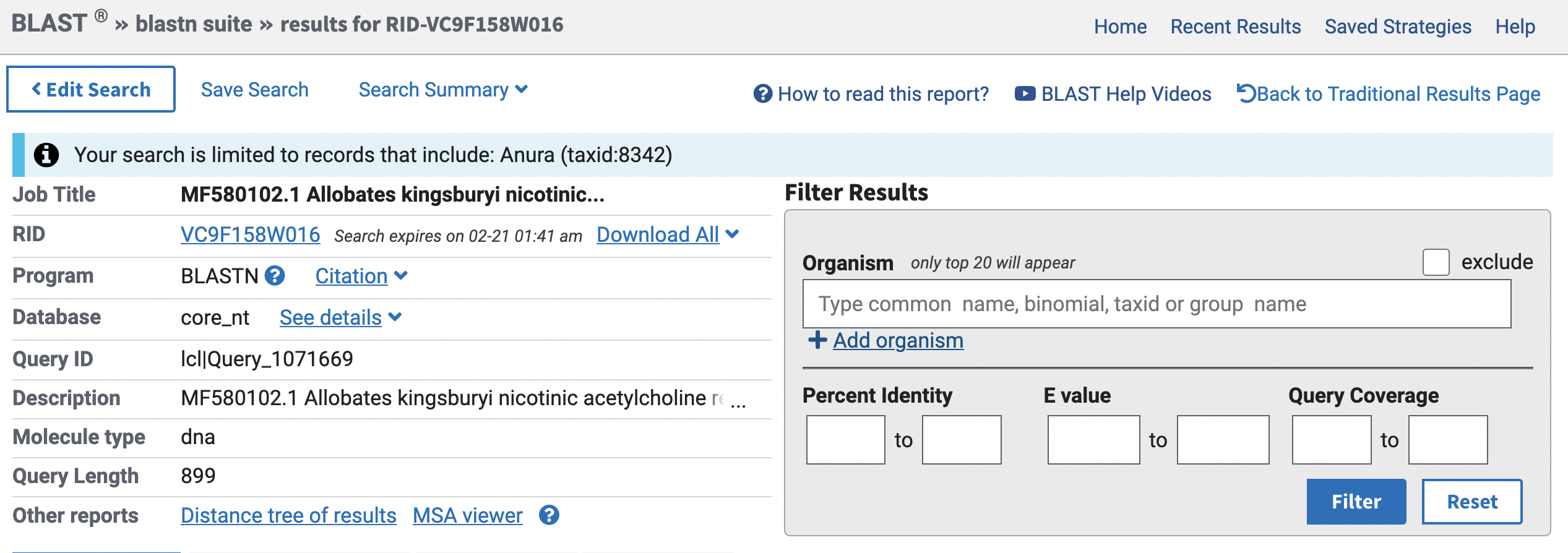
This provides an overview of your query, such title, program (e.g., blastn), type of molecule (e.g., DNA), query length. Below this section, you will find links to specific sequences that match your query, ranked from most to least similar.
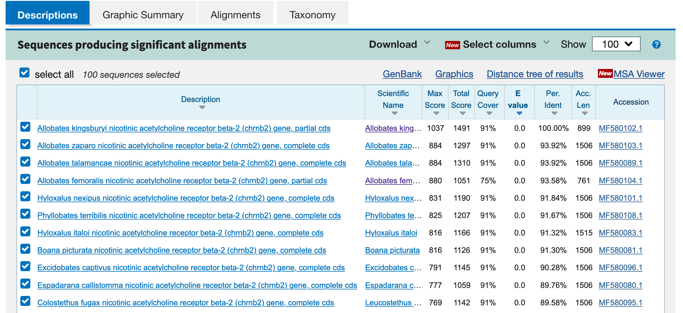
Some key information is provided here. The Descriptions will provided the name of the submission that matched your search. In this case, Allobates kingsburyi nicotinic acetylcholine receptor beta-2 (chrnb2) gene, partial cds is a perfect match because we searched this exact sequence. The matched are presented in order from the top as closets matches to the bottom as the worst. The three most important numbers that guide you in your reading of the results are: Query Cover – numbers close to 100% are preferred and 91% indicates that this percentage of the sequence in the query covered the sequence in description; E value – numbers close to 0 are preferred and in our case was 0 so it is an extremely close match and Per. Inden – numbers close to 100% are preferred and in our case is 100% or a perfect match.
Other relevant information is Accession or the number in the NCBI that you can retrieve using from R such as using rentrez.
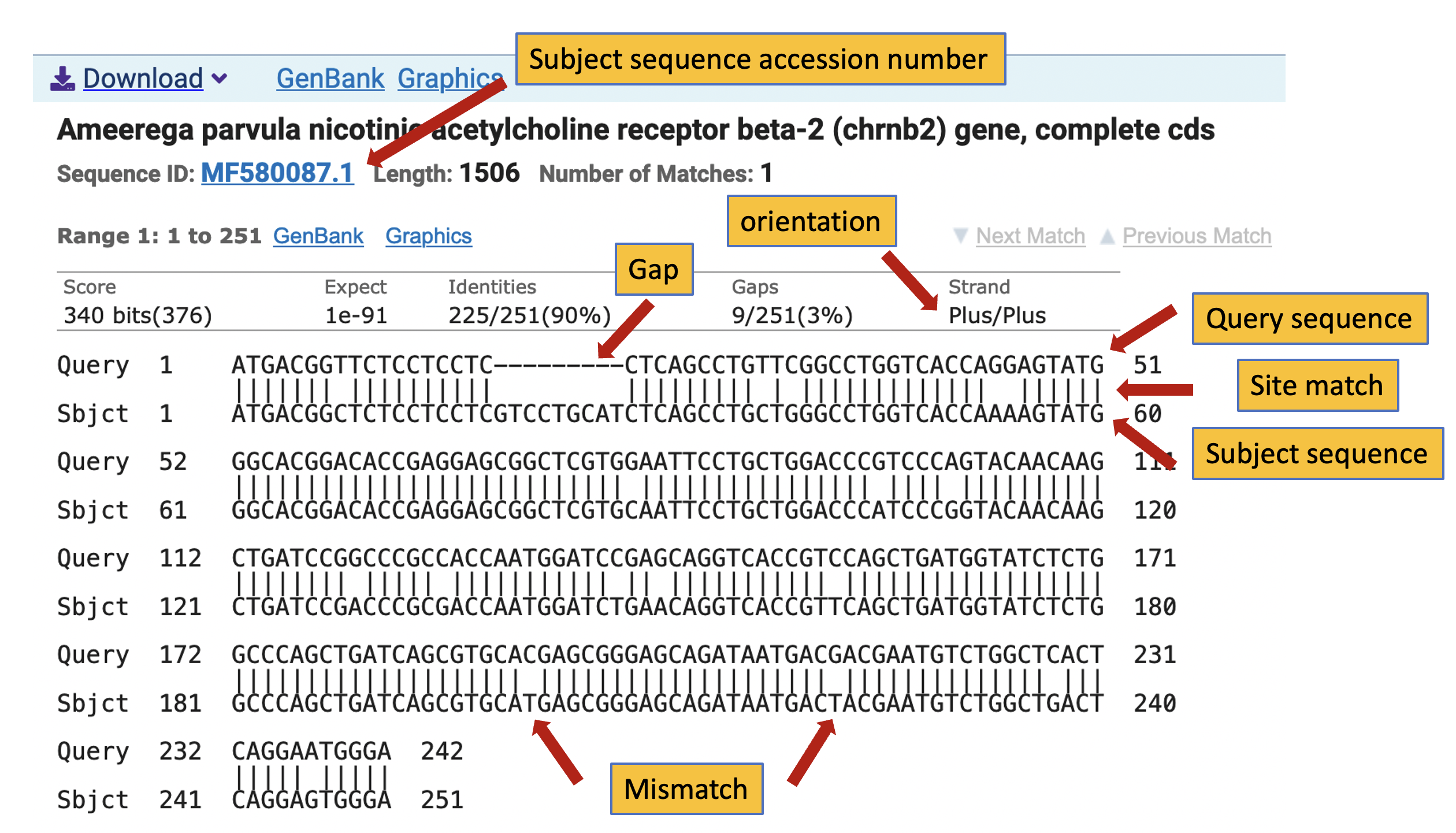
12) If you click on any of the matches or the Alignments tab, the browser will take you to the alignment. In there, you can find nucleotide sites that matched (i.e., Identities) or not.
The reading frame of the query as a Strand (e.g., Plus/Plus is standard; if Plus/Minus one needs to reverse and complement)
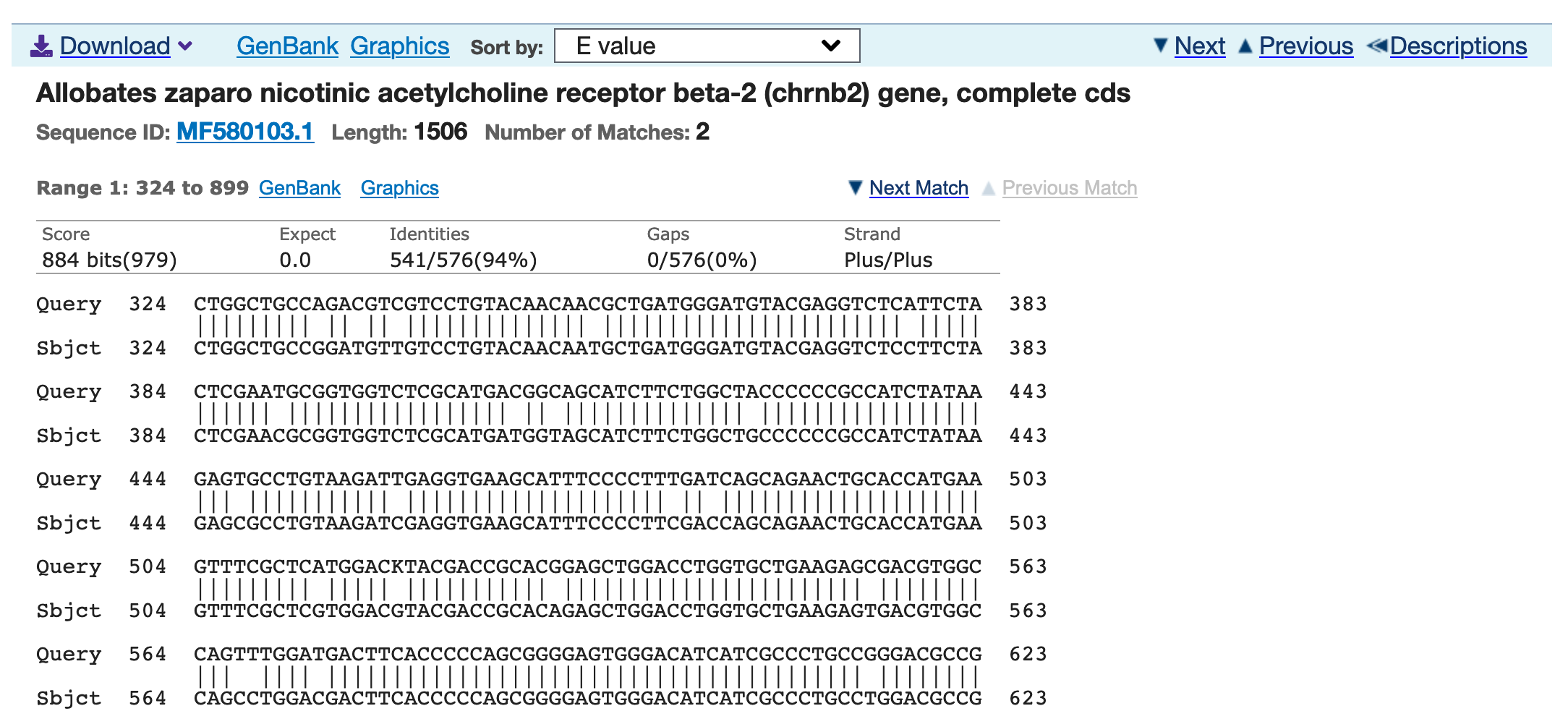
You can also click on the GenBank link to take you to the accession entry of the reference. In this case, MF580103.1 that is the sequence of Allobates zaparo.
13) From each alignment block, you can get a summary of how well the subject sequence matches your query. This includes the name of species, gene identity, and other information such if the subject sequence is complete (e.g., complete cds). It will also include the sequence ID or NCBI accession number and its length. On the alignment top row, you see the max score (‘Score’) and expect value (‘Expect’), a high score and very low expected values suggest a strong similarity to the query. The ‘Identities’ indicate the number of identical bases between the query and the subject sequences. The ‘Gaps’ indicate the number of gaps and their % in the alignment over the entire length of the matching section of the query versus the subject sequence alignment. The ‘Strand’ provides the orientation of the query sequence relative to the subject sequence. Such as Plus/Plus (both 3 -> 5), Minus/Minus (both 5 -> 3), and variations between these. Sometimes, you will see lowercase letters in the alignment (e.g., ‘ttttttttt’) these indicate low complexity sequences with lots of the same type of bases in the query sequence.
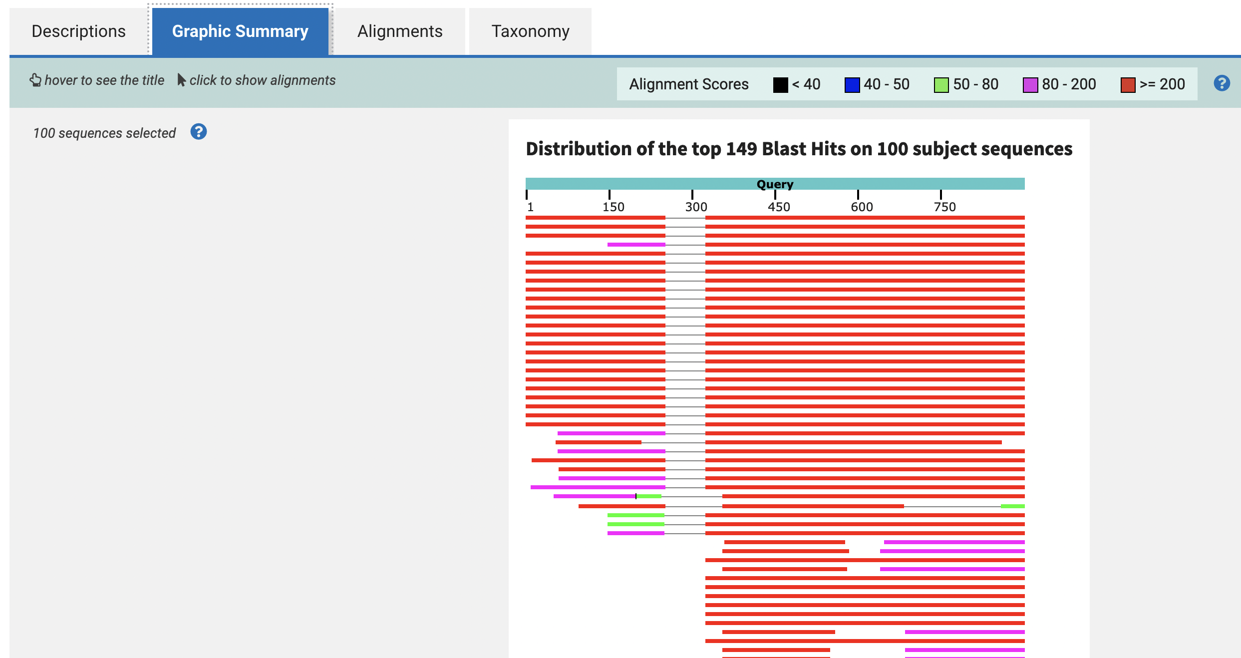
14) If you click on Graphic Summary this will show you the sequence alignments as colored lines that correspond to NCBI database matches to our query sequence. The light blue bar will indicate the nucleotide/amino acid position from 1 to the end. The matching sequences will present different colors based on the alignment scores to identify local regions of sequence similarity with the query sequence. Higher values (e.g., >= 200) would indicate higher similarity. You can notice that some aligned regions can be separated and connected by a thin grey line these are multiple alignment blocks. You can mouse over an alignment sequence to reveal the sequence title as in the NCBI database. Clicking on a line (i.e., alignment) will displays a box with more details about such alignment and a link to the sequence itself in the Alignments section of the report.
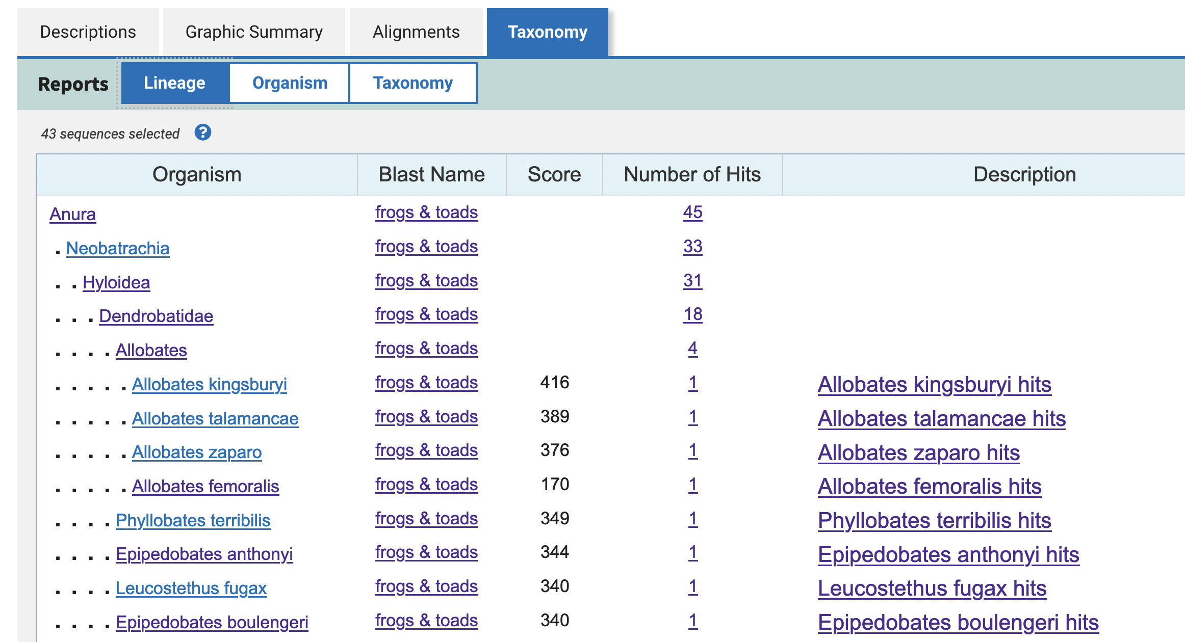
15) If you click on Taxonomy you will get a summary of the species source of the subject sequences (i.e., BLAST matches), including their higher taxonomic classification (e.g., family, class, order, etc).
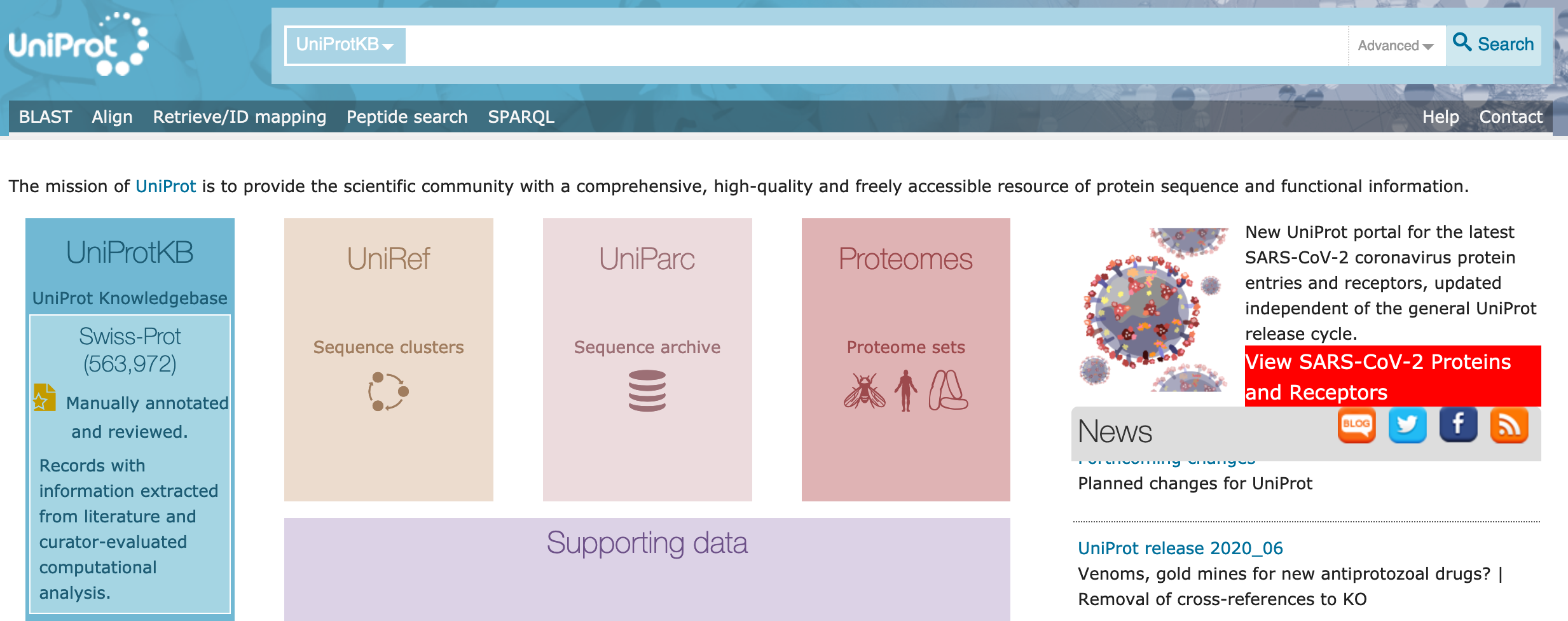
5.5 Other databases: UniProt
16) Other source of important sequence information is the UniProt database, which provides high-quality and freely accessible protein sequences and functional information.
 These sequences can be retrieved by their entry number using the R-package UniprotR. However, this package requires an additional one called GenomicAlignments available at Bioconductor,
#install and load the package
install.packages("UniprotR")

if (!require("BiocManager", quietly = TRUE))
    install.packages("BiocManager")

BiocManager::install("GenomicAlignments")
We can retrieve UniProt sequences of the same gene that presented before the acetylcholine receptor CHRNB2. For this purpose, we need to retrieve the list of entry numbers in the UniProt databases. For example, we will retrieve CHRNB2 from the following taxa: human P17787, mouse Q9ERK7, chicken P09484, Bos taurus A0A3Q1MJN8, Danio rerio E7F4S7, Coelacanth H3B5V5, Anolis H9GMJ0, Xenopus tropicalis A4IIS6.
We will use the function GetSequences().
# load required libraries
library(UniprotR)
library(GenomicAlignments)
library(Biostrings)

# retrieve sequences
other_CHRNB2_ids <- c("P17787", "Q9ERK7", "P09484", "A0A3Q1MJN8", "E7F4S7", "H3B5V5", "H9GMJ0", "A4IIS6")
other_CHRNB2_raw <- UniprotR::GetSequences(other_CHRNB2_ids)
class(other_CHRNB2_raw)
#[1] "data.frame"
# this is a complex data structure and we need the sequences that can be later process as AAStringSet
str(other_CHRNB2_raw)
#'data.frame':  8 obs. of  23 variables:
#$ Fragment                       : logi  NA NA NA NA NA NA ...
#$ Gene.encoded.by                : logi  NA NA NA NA NA NA ...
#$ Alternative.products..isoforms.: logi  NA NA NA NA NA NA ...
#$ Erroneous.gene.model.prediction: logi  NA NA NA NA NA NA ...
#$ Erroneous.initiation           : logi  NA NA NA NA NA NA ...
#$ Erroneous.termination          : logi  NA NA NA NA NA NA ...
#$ Erroneous.translation          : logi  NA NA NA NA NA NA ...
#$ Frameshift                     : logi  NA NA NA NA NA NA ...
#$ Mass.spectrometry              : logi  NA NA NA NA NA NA ...
#$ Polymorphism                   : logi  NA NA NA NA NA NA ...
#$ RNA.editing                    : logi  NA NA NA NA NA NA ...
#$ Sequence.caution               : logi  NA NA NA NA NA NA ...
#$ Length                         : int  502 501 491 509 543 478 509 499
#$ Mass                           : Factor w/ 8 levels "57,019","57,113",..: 1 2 3 4 5 6 7 8
#$ Sequence                       : Factor w/ 8 levels "MARRCGPVALLLGFGLLRLCSGVWGTDTEERLVEHLLDPSRYNKLIRPATNGSELVTVQLMVSLAQLISVHEREQIMTTNVWLTQEWEDYRLTWKPEEFDNMKKVRLPSKH"| __truncated__,..: 1 2 3 4 5 6 7 8
#$ Alternative.sequence           : logi  NA NA NA NA NA NA ...
#$ Natural.variant                : Factor w/ 1 level "VARIANT 287;  /note=V -> L (in ENFL3; dbSNP:rs74315291);  /evidence=ECO:0000269|PubMed:11062464;  /id=VAR_01271"| __truncated__: 1 NA NA NA NA NA NA NA
#$ Non.adjacent.residues          : logi  NA NA NA NA NA NA ...
#$ Non.standard.residue           : logi  NA NA NA NA NA NA ...
#$ Non.terminal.residue           : logi  NA NA NA NA NA NA ...
#$ Sequence.conflict              : Factor w/ 2 levels "CONFLICT 26;  /note=T -> A (in Ref. 4; CAA05108);  /evidence=ECO:0000305; CONFLICT 426;  /note=E -> A (in Ref. "| __truncated__,..: 1 2 NA NA NA NA NA NA
#$ Sequence.uncertainty           : logi  NA NA NA NA NA NA ...
#$ Version..sequence.             : int  1 2 1 1 1 1 1 1
We notice that from the above data frame, we only need the $ Sequence slot. However, this is a factor element and has to be transformed into vector. We will proceed as follows.
other_CHRNB2_aa <- other_CHRNB2_raw$Sequence
class(other_CHRNB2_aa)
#[1] "factor"
# we transform to a character vector
other_CHRNB2_aa <- as.character(other_CHRNB2_aa)
class(other_CHRNB2_aa)
other_CHRNB2_aa
#[1] "MARRCGPVALLLGFGLLRLCSGVWGTDTEERLVEHLLDPSRYNKLIRPATNGSELVTVQLMVSLAQLISVHEREQIMTTNVWLTQEWEDYRLTWKPEEFDNMKKVRL..."
#[2] "MARCSNSMALLFSFGLLWLCSGVLGTDTEERLVEHLLDPSRYNKLIRPATNGSELVTVQLMVSLAQLISVHEREQIMTTNVWLTQEWEDYRLTWKPEDFDNMKKVRL..."
#[3] "MALLRVLCLLAALRRSLCTDTEERLVEYLLDPTRYNKLIRPATNGSQLVTVQLMVSLAQLISVHEREQIMTTNVWLTQEWEDYRLTWKPEDFDNMKKVRLPSKHIWL..."
We notice that the and UniProt entries are not associated to the sequences and can get these names form the row names from the other_CHRNB2_raw data frame. By assigning such names, we can improve our ability to identify the source of the sequence by adding organism and the starting fasta character >. We can also prepare this object to build a fasta output by adding the corresponding new line character \n.
# get a names character vector
names_of_other_CHRNB2_aa <- rownames(other_CHRNB2_raw)
names_of_other_CHRNB2_aa
#[1] "P17787"     "Q9ERK7"     "P09484"     "A0A3Q1MJN8" "E7F4S7"     "H3B5V5"     "H9GMJ0"     "A4IIS6"
names_of_organism <- c("human", "mouse", "chicken", "Bos_taurus", "Danio_rerio", "coelacanth", "Anolis", "Xenopus_tropicalis")
# we can combine names
final_names <- character()
for(i in 1:length(names_of_organism)) { final_names[i] <- paste0(">",names_of_organism[i],"_",names_of_other_CHRNB2_aa[i],"\n")}
final_names
#[1] ">human_P17787\n"              ">mouse_Q9ERK7\n"              ">chicken_P09484\n"
#[4] ">Bos_taurus_A0A3Q1MJN8\n"     ">Danio_rerio_E7F4S7\n"        ">coelacanth_H3B5V5\n"
#[7] ">Anolis_H9GMJ0\n"             ">Xenopus_tropicalis_A4IIS6\n"
We can build the final FASTA output to be written in a text file. By collapsing both vectors with a new line character \n.
end_uniprot_fasta <- paste0(final_names,other_CHRNB2_aa, collapse = "\n")
end_uniprot_fasta
#[1] ">human_P17787\nMARRCGPVALLLGFGLLRLCSGVWGTDTEERLVEHLLDPSRYNKLIRPATNGSELVTVQLMVSLAQLISVHEREQIMTTNVWLTQEWEDYRLTWKPEEFDNMKKVRL..
cat(end_uniprot_fasta)
#>human_P17787
#MARRCGPVALLLGFGLLRLCSGVWGTDTEERLVEHLLDPSRYNKLIRPATNGSELVTVQLMVSLAQLISVHEREQIMTTNVWLTQEWEDYRLTWKPEEFDNMKKVRLPSKHIWLPDVVLYNNADGMY...
#>mouse_Q9ERK7
#MARCSNSMALLFSFGLLWLCSGVLGTDTEERLVEHLLDPSRYNKLIRPATNGSELVTVQLMVSLAQLISVHEREQIMTTNVWLTQEWEDYRLTWKPEDFDNMKKVRLPSKHIWLPDVVLYNNADGMY...
#>chicken_P09484
#MALLRVLCLLAALRRSLCTDTEERLVEYLLDPTRYNKLIRPATNGSQLVTVQLMVSLAQLISVHEREQIMTTNVWLTQEWEDYRLTWKPEDFDNMKKVRLPSKHIWLPDVVLYNNADGMYEVSFYSN...

# we write the output to a text file -- REMEMBER TO SET A PATH TO THE FOLDER THAT YOU WANT IN YOUR COMPUTER
name_of_file <- paste0("acetylcholine_receptor_Uniprot.txt")
name_of_file
#[1] "acetylcholine_receptor_popset_1248341763.txt"
write(end_uniprot_fasta, file = name_of_file)
Finally, we can import this updated file into R using Biostrings.
# get the path to the uniprot file with the amino acid sequences -- THIS IS EXCLUSIVE FOR YOUR COMPUTER AND IT IS NOT THE PATH SHOWN BELOW
my_uniprot_as_aa_stringset <- readAAStringSet(filepath = "~/Desktop/Teach_R/class_pages_reference/bioinformatics_gitbook_1/my_working_directory/acetylcholine_receptor_Uniprot.txt",
                                               format = "fasta")
my_uniprot_as_aa_stringset
#  A AAStringSet instance of length 8
#   width seq                                                                                       names
#[1]   502 MARRCGPVALLLGFGLLRLCSGVWGTDTEERLVEHLLDPSRYN...RLFLWIFVFVCVFGTIGMFLQPLFQNYTTTTFLHSDHSAPSSK human_P17787
#[2]   501 MARCSNSMALLFSFGLLWLCSGVLGTDTEERLVEHLLDPSRYN...RLFLWIFVFVCVFGTIGMFLQPLFQNYTATTFLHSDHSAPSSK mouse_Q9ERK7
#[3]   491 MALLRVLCLLAALRRSLCTDTEERLVEYLLDPTRYNKLIRPAT...RLFLWIFVFVCVFGTVGMFLQPLFQNYATNSLLQLGQGTPTSK chicken_P09484
#[4]   509 MAWLSGPKAMLLSFGLLGLCSGVWGTDTEERLVEHLLDPSRYN...FVCVFGTIGMFLQPLFQNYATATFLHADHSAPSSKCVLSPPEI Bos_taurus_A0A3Q1...
#[5]   543 MMALWTLFCILAIVKSGYGADTEERLVEHLLNPAHYNKLIRPA...VAMVIDRLFLWIFVFVCVFGTIGMFLQPLFQNYTAKTITHTPG Danio_rerio_E7F4S7
#[6]   478 SLAMDTEERLVGHLLNPAHYNKLIRPATNRSEVVTVQLMVSLA...MVIDRLFLWIFVFVCIFGTLGMFLQPVFQNSSFDSLPQKTNAA coelacanth_H3B5V5
#[7]   509 CAASSHFAACPASGSLLGLSAGVLGTDTEERLVEHLLDPLRYN...RLFLWIFVFVCVFGTIGMFLQPLFQNYATNSLLQIHQGAPGSK Anolis_H9GMJ0
#[8]   499 MIRTGMAPLLAALYLLLGLLPGCLGTDTEERLVEHLLDPSRYN...VIDRLFLWIFVFVCVFGTIGMFLQPLFQNYTTNALVHMNHAAN Xenopus_tropicali...
17) We can also append both AAStringSets: my_protein_as_aa_stringset and my_uniprot_as_aa_stringset for further downstream analyses with the function c().
all_aa_stringset <- c(my_protein_as_aa_stringset, my_uniprot_as_aa_stringset)
all_aa_stringset
#AAStringSet object of length 29:
#     width seq                                                                                                                      names
# [1]   501 MTVLLXXXXLGLLGLVTRCLXTDTEERLVEFLLDSSRYNKLIRPATNGSEQVTVQLMVS...QSVSEDWKYVAMVIDRLFLWIFVFVCVFGTIGMFLQPLFQNYTTNTLLQLNHAAPASN ATG31782.1 nicoti...
# [2]    65 ADGMYEVSFYSNAVVSHDGSIFWLPPAIYKSACKIEVKHFPFDQQNCTMKFRSWTYDRTELDLVL                                                        ATG31811.1 nicoti...
# [3]   501 MTALLLVLHLSLLGLVTRSMGTDTEERLVEFLLDPSRYNKLIRPATNGSEQVTVQLMVS...QSVSEDWKYVAMVIDRLFLWIFVFVCVFGTIGMFLQPLFQNYTSNTLIQLNHGTPASN ATG31810.1 nicoti...
# [4]    67 ADGMYEVSFYSNAVVSHDGSIFWLPPAIYKSACKIEVKHFPFDQQNCTMKFRSWTYDRTELDLVLKS                                                      ATG31809.1 nicoti...
# [5]    44 ADGMYEVSFYSNAVVSHDGSIFWLPPAIYKSACKIEVKHFPFDQ                                                                             ATG31808.1 nicoti...
# ...   ... ...
#[25]   509 MAWLSGPKAMLLSFGLLGLCSGVWGTDTEERLVEHLLDPSRYNKLIRPATNGSELVTVQ...YVAMVIDRLFLWIFVFVCVFGTIGMFLQPLFQNYATATFLHADHSAPSSKCVLSPPEI Bos_taurus_A0A3Q1...
#[26]   543 MMALWTLFCILAIVKSGYGADTEERLVEHLLNPAHYNKLIRPATNGSEVVTVQLMVSLA...KSEDDDRSVSEDWKYVAMVIDRLFLWIFVFVCVFGTIGMFLQPLFQNYTAKTITHTPG Danio_rerio_E7F4S7
#[27]   478 SLAMDTEERLVGHLLNPAHYNKLIRPATNRSEVVTVQLMVSLAQLISVHERAQIMTTNC...EDKKRSVIEDWKYVAMVIDRLFLWIFVFVCIFGTLGMFLQPVFQNSSFDSLPQKTNAA coelacanth_H3B5V5
#[28]   509 CAASSHFAACPASGSLLGLSAGVLGTDTEERLVEHLLDPLRYNKLIRPATNGSELVTVQ...QSVSEDWKYVAMVIDRLFLWIFVFVCVFGTIGMFLQPLFQNYATNSLLQIHQGAPGSK Anolis_H9GMJ0
#[29]   499 MIRTGMAPLLAALYLLLGLLPGCLGTDTEERLVEHLLDPSRYNKLIRPATNGSEQVTVQ...DDDQSVSEDWKYVAMVIDRLFLWIFVFVCVFGTIGMFLQPLFQNYTTNALVHMNHAAN Xenopus_tropicali...
5.6 Other databases: Ensembl
Ensembl is an online archive for vertebrate genomes that are used in comparative genomics, evolution, sequence variation and transcriptional regulation. Ensembl is quite extensive and convoluted to access and export data.
The R-package biomaRt provides a somehow easy access to datasets present or crosslinked with Ensembl.
18) We will illustrate how to access the acetylcholine receptor CHRNB2 sequence in the genome of Xenopus tropicalis frog model system.
First, you might need to install biomaRt from Bioconductor.
BiocManager::install("biomaRt")
library(biomaRt)
We can get a list to which biomaRt can connect using the function listMarts().
listMarts()
#               biomart                version
#1 ENSEMBL_MART_ENSEMBL      Ensembl Genes 102
#2   ENSEMBL_MART_MOUSE      Mouse strains 102
#3     ENSEMBL_MART_SNP  Ensembl Variation 102
#4 ENSEMBL_MART_FUNCGEN Ensembl Regulation 102
We can also type ensembl using the function useMart() to access all accessible databases.
mart <- useMart('ensembl')
# this will give you at least 203 dataset to search
listDatasets(mart)
#                           dataset                                                  description                           version
#1         acalliptera_gene_ensembl                             Eastern happy genes (fAstCal1.2)                        fAstCal1.2
#2       acarolinensis_gene_ensembl                               Anole lizard genes (AnoCar2.0)                         AnoCar2.0
#3        acchrysaetos_gene_ensembl                              Golden eagle genes (bAquChr1.2)                        bAquChr1.2
#4        acitrinellus_gene_ensembl                               Midas cichlid genes (Midas_v5)                          Midas_v5
#5        amelanoleuca_gene_ensembl                                        Panda genes (ailMel1)                           ailMel1
#...
For our example, we will use the Xenopus tropicalis dataset named in the list above as "xtropicalis_gene_ensembl". However, we need to be more specific how we want to search that database. For that purpose, we can use the function listFilters() to list the filters available in our selected dataset.
xenopus_mart <- useMart("ensembl", dataset="xtropicalis_gene_ensembl")
listFilters(xenopus_mart)
#                              name                                                      description
#1                  chromosome_name                                         Chromosome/scaffold name
#2                            start                                                            Start
#3                              end                                                              End
#4                           strand                                                           Strand
#5               chromosomal_region                           e.g. 1:100:10000:-1, 1:100000:200000:1
#6       with_entrezgene_trans_name                            With EntrezGene transcript name ID(s)
#7                        with_embl                           With European Nucleotide Archive ID(s)
#8                with_arrayexpress                                      With Expression Atlas ID(s)
#9                          with_go                                                    With GO ID(s)
#...
We will retrieve based on the name of gene in UniProt (i.e., CHRNB2) so two filter seem to be useful based on the description column hgnc_symbol and uniprot_gn_symbol. We will try to retrieve such gene sequence using the function getSequence().
xenopus_CHRNB2_seq_hgnc_symbol <- getSequence(id = "chrnb2",
                                            type = "uniprot_gn_symbol",
                                         seqType = "peptide",
                                            mart = xenopus_mart)

xenopus_CHRNB2_seq_uniprot_id <- getSequence(id = "A4IIS6",
                                            type = "uniprot_gn_id",
                                         seqType = "peptide",
                                            mart = xenopus_mart, verbose = TRUE)


show(xenopus_CHRNB2_seq_uniprot_id)
5.7 Other databases: Taxonomy, phylogenetic trees and species distributions
Accessing other biological repositories through R is in some cases a hit-and-miss. Some with stand and be reliable, but the depend on the source database.
Here is a list of some R-packages and the databases that you can access. Most of these will have vignettes for you to follow:
- taxize – Taxonomic Information from Around the Web.
- BIEN – Tools for Accessing the Botanical Information and Ecology Network Database.
- rotl – Interface to the ‘Open Tree of Life’ API.
- rgbif – Interface to the Global ‘Biodiversity’ Information Facility API.
- rvertnet – Search ‘Vertnet’, a ‘Database’ of Vertebrate Specimen Records.
- spocc – Interface to Species Occurrence Data Sources.