Session 32 – Miscellaneous
We will post miscellaneous code developed during class or requested by you in this chapter. We will keep updating this list as the semester progresses.
32.1 Sampling from a vector of names
We need that 2-3 students give a presentation about the topics of previous class every week, so we can use R to do the selection for us. We will use the function sample
## We need a list of the 17 students last names for BIO/BIT 209 as their unique identifiers

students_BIO209 <- c("Ardire", "Carlucci", "Da_Costa_Morais", "Davidov", "Deda",
                     "Dimitrijevic", "Fasano",  "Javed", "Mahadeo", "Mowla", "Njie",
                     "Rahman", "Siddique", "Sukhram","Tan", "Tiumalu", "Vu")

students_BIO209
#[1] "Ardire"          "Carlucci"        "Da_Costa_Morais" "Davidov"         "Deda"
#[6] "Dimitrijevic"    "Fasano"          "Javed"           "Mahadeo"         "Mowla"
#[11] "Njie"            "Rahman"          "Siddique"        "Sukhram"         "Tan"
#[16] "Tiumalu"         "Vu"

## we order them alphabetically

students_BIO209_order <- sort(students_BIO209)
students_BIO209_order
#[1] "Ardire"          "Carlucci"        "Da_Costa_Morais" "Davidov"         "Deda"
#[6] "Dimitrijevic"    "Fasano"          "Javed"           "Mahadeo"         "Mowla"
#[11] "Njie"            "Rahman"          "Siddique"        "Sukhram"         "Tan"
#[16] "Tiumalu"         "Vu"

## numeric code for each student
students_BIO209_order_c <- paste(1:17, students_BIO209_order, sep = "_")
students_BIO209_order_c
#[[1] "1_Ardire"          "2_Carlucci"        "3_Da_Costa_Morais" "4_Davidov"         "5_Deda"
#[6] "6_Dimitrijevic"    "7_Fasano"          "8_Javed"           "9_Mahadeo"         "10_Mowla"
#[11] "11_Njie"           "12_Rahman"         "13_Siddique"       "14_Sukhram"        "15_Tan"
#[16] "16_Tiumalu"        "17_Vu"

## we sample 2 students to give a review of last class

todays_2_students_code <- sample(1:17, size = 2, replace = FALSE, prob = NULL)
todays_2_students_code
#[1] 16 13

## we identify such students by name

today_students <- students_BIO209_order_c[todays_2_students_code]
today_students
#[1] "16_Tiumalu"  "13_Siddique"

## NEXT WEEK: we need 2 students again, but we want to remove those that already gave a lesson

remaining_students_code <- setdiff(1:17, c(16,13))
remaining_students_code
#[1]  1  2  3  4  5  6  7  8  9 10 11 12 14 15 17

## NEXT WEEK: we sample 2 students to give a review of last class

todays_2_students_code <- sample(remaining_students_code, size = 2, replace = FALSE, prob = NULL)
todays_2_students_code
#[1]  7 15

## NEXT WEEK: we identify such students by name

today_students <- students_BIO209_order_c[todays_2_students_code]
today_students
#[1] "7_Fasano" "15_Tan"
32.2 Read a text from an article pdf
We can often summarize a pdf of paper or article using a world cloud. For this purpose, we need to read a pdf from our desktop using the R-package pdftools and read the text to a vector using tm: Text Mining Package.
## We need to install and load some R-packages
install.packages("pdftools")
library(pdftools)
install.packages("tm")
library(tm)

## file path to my pdf file
my_pdf_file_path <- "~/Desktop/Teach_R/class_pages_reference/bioinformatics_gitbook_1/my_working_directory/Almeida_Paiva_etal_2022.pdf"

## read pdf text to a vector
pdf_text <- pdf_text(my_pdf_file_path, opw = "", upw = "")

## remove special characters like "–"

pdf_text <- gsub("–"," ", pdf_text)

## create a text vector from pdf text and remove unwanted characters

docs <- Corpus(VectorSource(pdf_text))
docs <- tm_map(docs, removeNumbers)
docs <- tm_map(docs, removePunctuation)
docs <- tm_map(docs, stemming)
docs <- tm_map(docs, stripWhitespace)
docs <- tm_map(docs, content_transformer(tolower))
my_pdf_corpus <- tm_map(docs, removeWords, stopwords("english"))

my_pdf_corpus
#<<SimpleCorpus>>
#Metadata:  corpus specific: 1, document level (indexed): 0
#Content:  documents: 28

## we process the my_text_pdf to a term-document matrix (tdm or TDM). This TDM stores counts of terms for the pdf document using the tm function 'TermDocumentMatrix'.

my_pdf_corpus_tdm <- TermDocumentMatrix(my_pdf_corpus)

inspect(my_pdf_corpus_tdm)
#<<TermDocumentMatrix (terms: 4796, documents: 28)>>
#Non-/sparse entries: 9858/124430
#Sparsity           : 93%
#Maximal term length: 50
#Weighting          : term frequency (tf)
#Sample             :
#             Docs
#Terms         16  2 20 21 24 25 26  3  5  8
#  available    5  5  4  6  0  0  0  4  4  8
#  can          6  9  8  7  1  0  0  6  8 13
#  free         2  0  1  2  0  0  0  0  3  2
#  information  6  1  4  7  0  0  1  0  2  4
#  molecular    0  4  0  3  3  7  0  6 14 14
#  protein     50 13 18 15  1  0  5 18  4  3
#  proteins     8  7  8  3  2  3  2  2  3  2
#  structure    1  6  6  7  1  0  2  2  1  4
#  structures   5  7  6  5  0  0  0  6  1  7
#  tool        13  8  5  8  0  0  1  4  9  9

## we create a matrix of word as a dataframe to be analyzed

pdf_matrix <- as.matrix(my_pdf_corpus_tdm)
pdf_words <- sort(rowSums(pdf_matrix),decreasing=TRUE)
pdf_df_for_map <- data.frame(word = names(pdf_words),freq=pdf_words)
head(pdf_df_for_map)

#               word freq
#protein     protein  260
#can             can  143
#available available  127
#tool           tool  124
#proteins   proteins   98
#molecular molecular   92
32.3 Read a text from a website
We can often summarize a website using a world cloud. For example, the page on Wikipedia corresponding to bioinformatics.
## We need to install and load some R-packages
install.packages("htm2txt")
library(htm2txt)

## create a vector with our selected url (website link address)
url <- 'https://en.wikipedia.org/wiki/Bioinformatics'

## get the text on the website as a vector
my_text_url <- gettxt(url)
my_text_url

## remove some garbage symbols like •
my_text_url <- gsub("•","",my_text_url)

## create a text vector from pdf text and remove unwanted characters

docs <- Corpus(VectorSource(my_text_url))
docs <- tm_map(docs, removeNumbers)
docs <- tm_map(docs, removePunctuation)
docs <- tm_map(docs, stemming)
docs <- tm_map(docs, stripWhitespace)
docs <- tm_map(docs, content_transformer(tolower))
my_url_corpus <- tm_map(docs, removeWords, stopwords("english"))

my_url_corpus
#<<SimpleCorpus>>
#Metadata:  corpus specific: 1, document level (indexed): 0
#Content:  documents: 1

## we process the my_url_corpus to a term-document matrix (tdm or TDM). This TDM stores counts of terms for the url document using the tm function 'TermDocumentMatrix'.

my_url_corpus_tdm <- TermDocumentMatrix(my_url_corpus)

inspect(my_url_corpus_tdm)
#<<TermDocumentMatrix (terms: 2709, documents: 1)>>
#Non-/sparse entries: 2709/0
#Sparsity           : 0%
#Maximal term length: 52
#Weighting          : term frequency (tf)
#Sample             :
#                Docs
#Terms              1
#  analysis        74
#  bioinformatics 126
#  biology        112
#  computational   66
#  data            70
#  gene            48
#  genome          52
#  information     49
#  protein         76
#  sequence        62

## we create a matrix of word as a dataframe to be analyzed

url_matrix <- as.matrix(my_url_corpus_tdm)
url_words <- sort(rowSums(url_matrix),decreasing=TRUE)
url_df_for_map <- data.frame(word = names(url_words),freq=url_words)
head(url_df_for_map)

#                          word freq
#bioinformatics bioinformatics  126
#biology               biology  112
#protein               protein   76
#analysis             analysis   74
#data                     data   70
#computational   computational   66
32.4 Read a text from a file
We can often summarize a text file using a world cloud. For example, your CANVAS responses about this bioinformatic class. Here is an text derived from this paper Ten simple rules for biologists learning to program by Maureen A. Carey and Jason A. Papin.
## my path to my text file

my_text_file <- '~/Desktop/Teach_R/class_pages_reference/bioinformatics_gitbook_1/my_working_directory/Carey_Papin_2018_text.txt'

## read text file as a vector
my_text <- paste(readLines(my_text_file),collapse=" ")
my_text

## remove some garbage symbols like •
my_text <- gsub("•","",my_text)

## create a text vector from pdf text and remove unwanted characters

docs <- Corpus(VectorSource(my_text))
docs <- tm_map(docs, removeNumbers)
docs <- tm_map(docs, removePunctuation)
docs <- tm_map(docs, stemming)
docs <- tm_map(docs, stripWhitespace)
docs <- tm_map(docs, content_transformer(tolower))
my_text_corpus <- tm_map(docs, removeWords, stopwords("english"))

my_text_corpus
#<<SimpleCorpus>>
#Metadata:  corpus specific: 1, document level (indexed): 0
#Content:  documents: 1

## we process the my_text_corpus to a term-document matrix (tdm or TDM). This TDM stores counts of terms for the text vector using the tm function 'TermDocumentMatrix'.

my_text_corpus_tdm <- TermDocumentMatrix(my_text_corpus)

inspect(my_text_corpus_tdm)
#<<<TermDocumentMatrix (terms: 1255, documents: 1)>>
#Non-/sparse entries: 1255/0
#Sparsity           : 0%
#Maximal term length: 70
#Weighting          : term frequency (tf)
#Sample             :
#               Docs
#Terms            1
#  biology       18
#  can           15
#  code          14
#  computational 30
#  data          18
#  language      21
#  languages     19
#  learn         14
#  rules         17
#  simple        16

## we create a matrix of word as a dataframe to be analyzed

text_matrix <- as.matrix(my_text_corpus_tdm)
text_words <- sort(rowSums(text_matrix),decreasing=TRUE)
text_df_for_map <- data.frame(word = names(text_words),freq=text_words)
head(text_df_for_map)

#                       word freq
#computational computational   30
#language           language   21
#languages         languages   19
#biology             biology   18
#data                   data   18
#rules                 rules   17
32.5 Generate the word cloud
There are many visual and descriptive representation or summaries of text data, which usually involve a presentation of key words (e.g., those used more frequently) on text, books, tweets, websites, etc. We can use a world cloud to summarize the frequency of single words, and the importance of each world could be shown with its font size and color. Three main reasons to use a world cloud might include: (1) To present text data in a clear and simple format, (2) To communicate basic insights based on a large corpus of text (e.g., a speech, a publication, a book, a website), and (3) To visually engage an audience so they can get the gist (i.e., essence or the main point) and draw insights quickly and, at the same time, allowing for some flexibility in their interpretation. For more insight see these links: Céline Van den Rul and here. We need to read text from a file, pdf, website as indicated previously. There are many online word-cloud, but for this course we use two R-packages: wordcloud and wordcloud2
## We need to install and load some R-packages
install.packages("wordcloud")
library(wordcloud)
install.packages("wordcloud2")
library(wordcloud2)
32.6 worldcloud – PDF
set.seed(1234) # for reproducibility
wordcloud(words = pdf_df_for_map$word,
           freq = pdf_df_for_map$freq,
       min.freq = 2,
      max.words = 100,
   random.order = FALSE,
        rot.per = 0.35,
         colors = brewer.pal(9, "Set1"))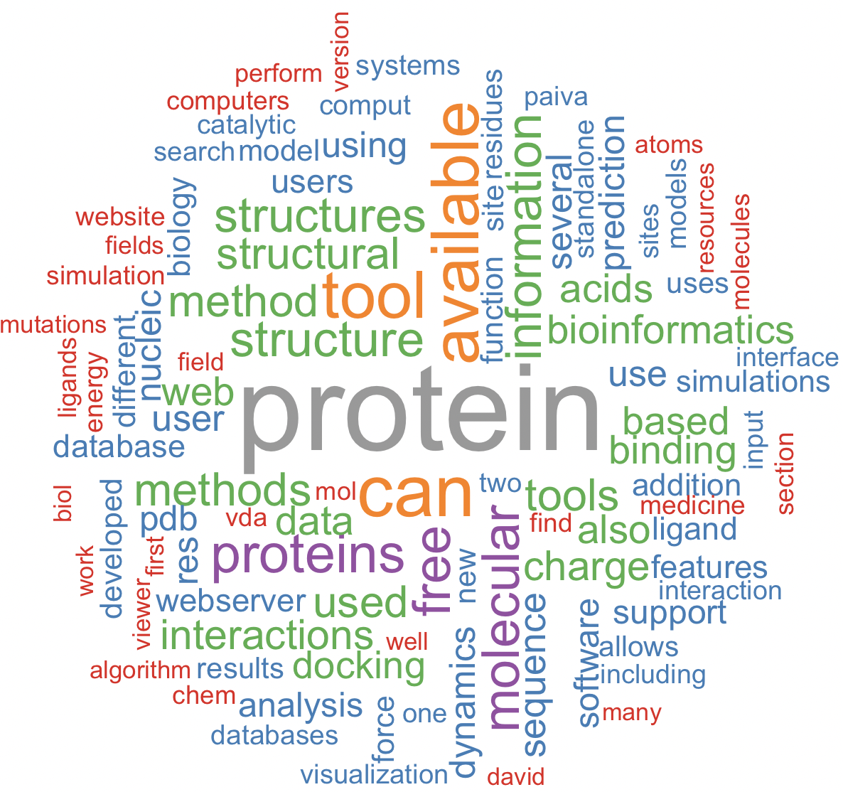
We can also use wordcloud2, which has more options and opens in a browser.
wordcloud2(data=pdf_df_for_map, size = 1, color = "random-light", backgroundColor = "white")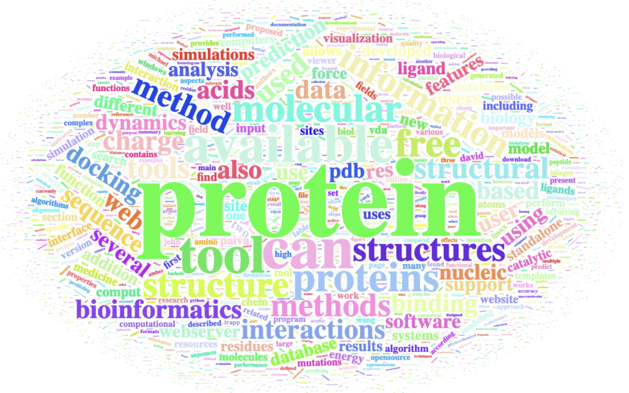
32.7 Worldcloud – website
set.seed(1234) # for reproducibility

wordcloud(words = url_df_for_map$word,
           freq = url_df_for_map$freq,
       min.freq = 2,
      max.words = 100,
   random.order = FALSE,
         colors = brewer.pal(7, "Accent"))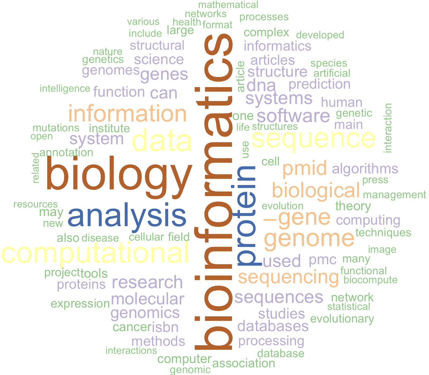
We can also use wordcloud2, which has more options and opens in a browser.
wordcloud2(data=url_df_for_map, size = 0.6, color='random-dark', shape = 'diamond', backgroundColor = "grey")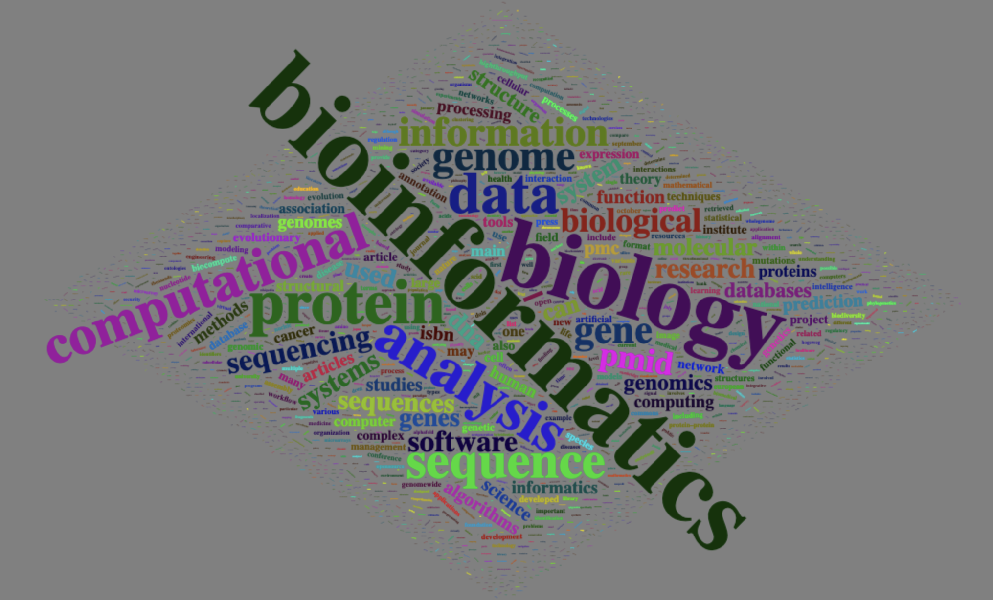
32.8 Worldcloud – text
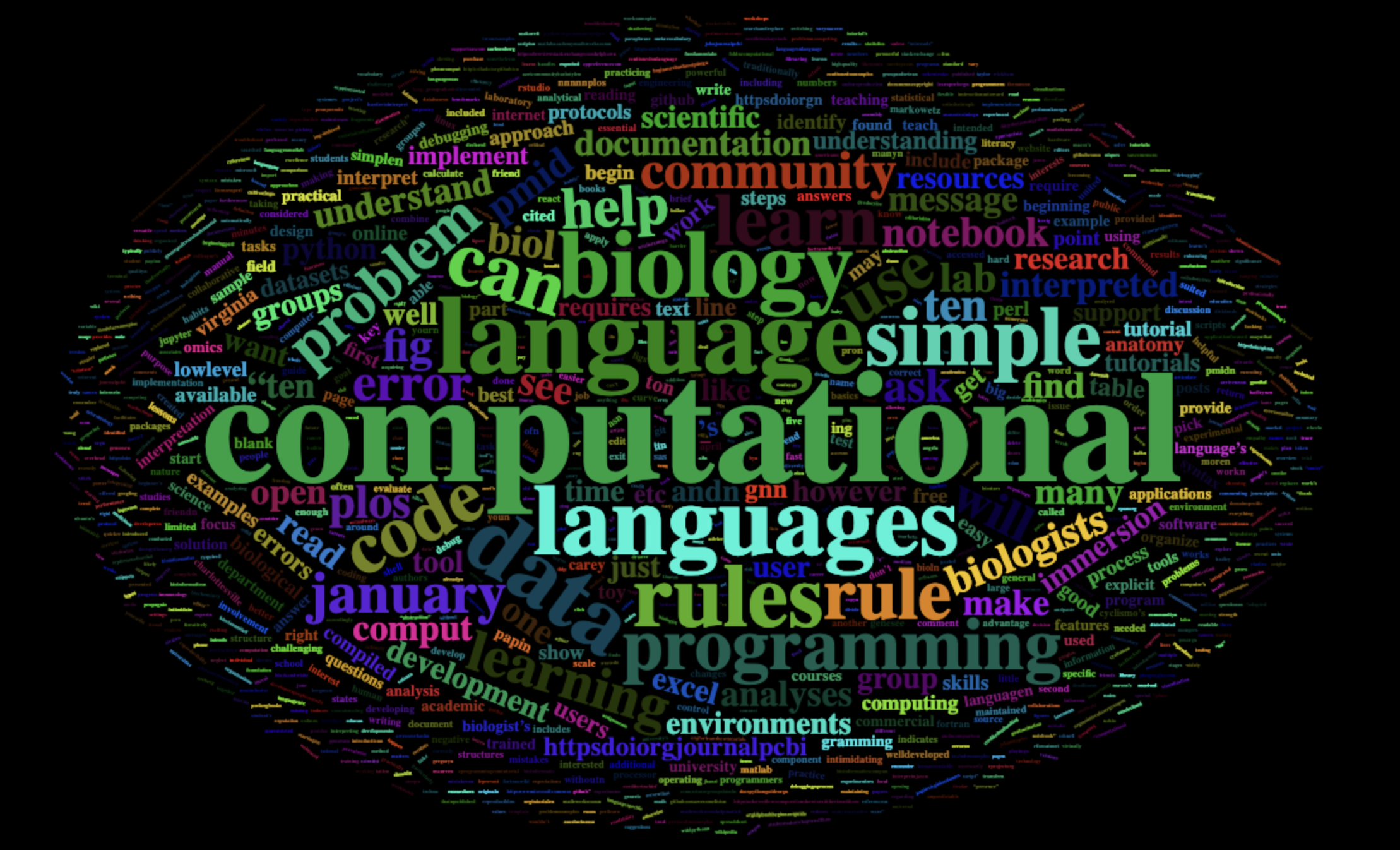
set.seed(1234) # for reproducibility

wordcloud(words = text_df_for_map$word,
           freq = text_df_for_map$freq,
       min.freq = 2,
      max.words = 100,
   random.order = FALSE,
        rot.per = 0.35,
         colors = brewer.pal(7, "Dark2"))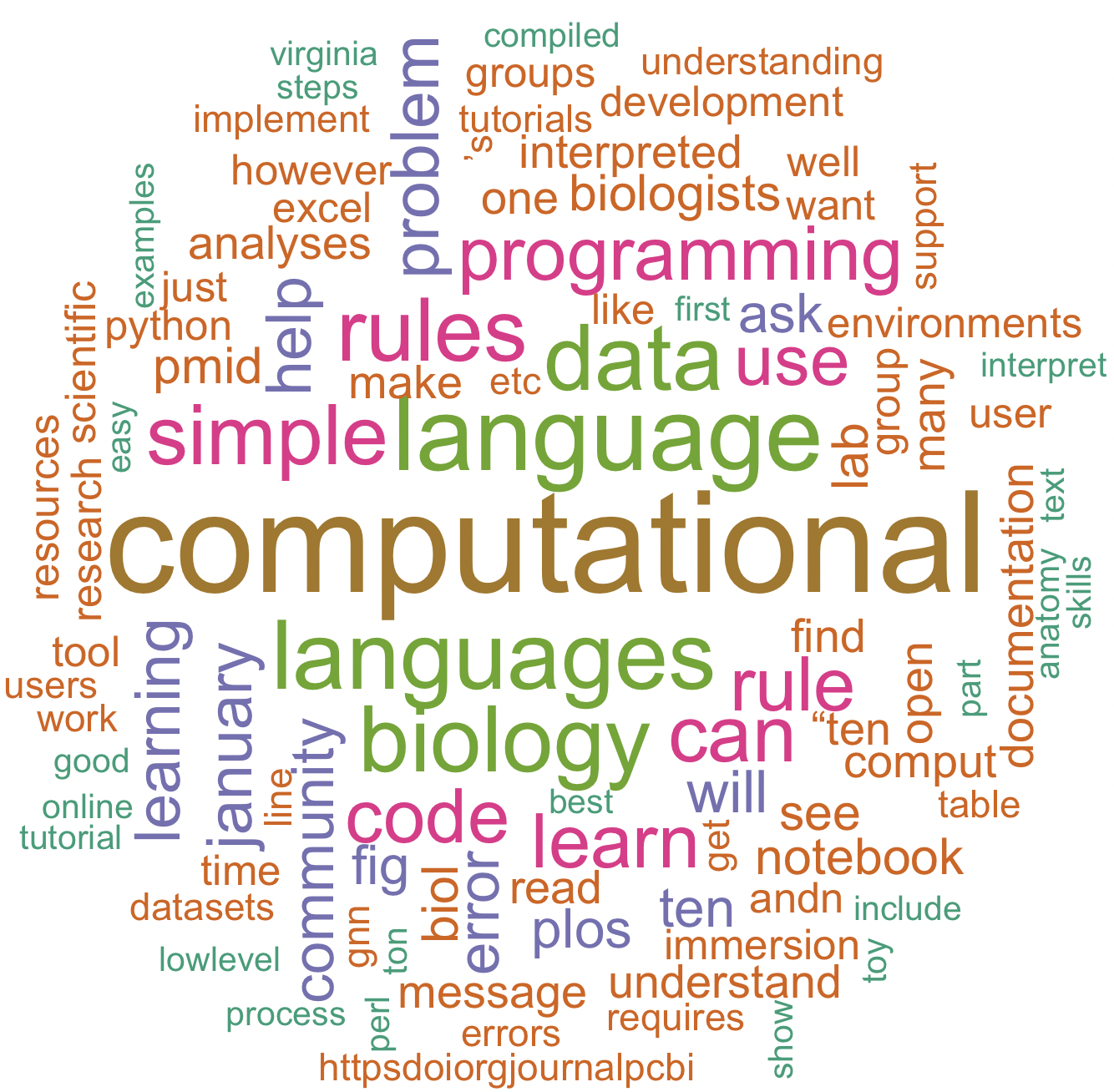
We can also use wordcloud2, which has more options and opens in a browser.
wordcloud2(data=text_df_for_map, size = 0.7, color='random-dark', backgroundColor = "black")