Session 6 – Basic Statistics in R
This workshop is not designed to give you an extensive overview on all statistical methods that can be performed in R. Yet, this computing environment was born to provide a comprehensive platform for the implementation of statistical methods. We will overview of some basic and advanced methods with some illustrative graphs (these will be expanded in the session devoted to graphics). However, you can ask me if you want to explore a specific method that you would me to add to this gitbook.
6.1 Exploring your data
1) To start, we need to import a dataset that we want to explore and analyze.
As graduate students, you are encouraged to use your own datasets (i.e., this is ideal as you will know more about its contents, metrics and intended use). For this exercise, I will use two previously show datasets: (1) the small preloaded mtcars dataset and (2) the large airway_scaledcounts.csv dataset. These datasets are in our class GitHub repository and you can download those to your computer.
## NOTE: remember to update the path to files with the datasets where you downloaded in your computer -- THIS IS EXCLUSIVE TO YOUR COMPUTER AND IT IS NOT THE PATH SHOWN BELOW

#define a working directory
setwd("~/Desktop/Teach_R/class_pages_reference/bioinformatics_gitbook_1/my_working_directory")
#load get mtcars dataset -- this a preloaded dataset in R
cars_data <- mtcars
cars_data
#                     mpg cyl  disp  hp drat    wt  qsec vs am gear carb
#Mazda RX4           21.0   6 160.0 110 3.90 2.620 16.46  0  1    4    4
#Mazda RX4 Wag       21.0   6 160.0 110 3.90 2.875 17.02  0  1    4    4
#Datsun 710          22.8   4 108.0  93 3.85 2.320 18.61  1  1    4    1
#Hornet 4 Drive      21.4   6 258.0 110 3.08 3.215 19.44  1  0    3    1
#...
#load get 'airway_scaledcounts.csv' dataset
airway_data <- read.table("~/Desktop/Teach_R/class_pages_reference/bioinformatics_gitbook_1/my_working_directory/airway_scaledcounts.csv",
               header = TRUE, sep = ",", stringsAsFactors = FALSE)
head(airway_data)
#          ensgene SRR1039508 SRR1039509 SRR1039512 SRR1039513 SRR1039516 SRR1039517 SRR1039520 SRR1039521
#1 ENSG00000000003        723        486        904        445       1170       1097        806        604
#2 ENSG00000000005          0          0          0          0          0          0          0          0
#3 ENSG00000000419        467        523        616        371        582        781        417        509
#4 ENSG00000000457        347        258        364        237        318        447        330        324
#5 ENSG00000000460         96         81         73         66        118         94        102         74
#6 ENSG00000000938          0          0          1          0          2          0          0          0
#...
2) We can get some basic descriptive parameters of each data set including number of entries, number and names of the columns (i.e., variables), type of variables (e.g., numbers or characters), number of NA values.
For this purpose, the easiest approach is to use the function summary()
summary(cars_data)
#     mpg             cyl             disp             hp             drat             wt             qsec             vs
# Min.   :10.40   Min.   :4.000   Min.   : 71.1   Min.   : 52.0   Min.   :2.760   Min.   :1.513   Min.   :14.50   Min.   :0.0000
# 1st Qu.:15.43   1st Qu.:4.000   1st Qu.:120.8   1st Qu.: 96.5   1st Qu.:3.080   1st Qu.:2.581   1st Qu.:16.89   1st Qu.:0.0000
# Median :19.20   Median :6.000   Median :196.3   Median :123.0   Median :3.695   Median :3.325   Median :17.71   Median :0.0000
# Mean   :20.09   Mean   :6.188   Mean   :230.7   Mean   :146.7   Mean   :3.597   Mean   :3.217   Mean   :17.85   Mean   :0.4375
# 3rd Qu.:22.80   3rd Qu.:8.000   3rd Qu.:326.0   3rd Qu.:180.0   3rd Qu.:3.920   3rd Qu.:3.610   3rd Qu.:18.90   3rd Qu.:1.0000
# Max.   :33.90   Max.   :8.000   Max.   :472.0   Max.   :335.0   Max.   :4.930   Max.   :5.424   Max.   :22.90   Max.   :1.0000
#       am              gear            carb
# Min.   :0.0000   Min.   :3.000   Min.   :1.000
# 1st Qu.:0.0000   1st Qu.:3.000   1st Qu.:2.000
# Median :0.0000   Median :4.000   Median :2.000
# Mean   :0.4062   Mean   :3.688   Mean   :2.812
# 3rd Qu.:1.0000   3rd Qu.:4.000   3rd Qu.:4.000
# Max.   :1.0000   Max.   :5.000   Max.   :8.000
summary(airway_data)
#   ensgene            SRR1039508         SRR1039509         SRR1039512         SRR1039513         SRR1039516
# Length:38694       Min.   :     0.0   Min.   :     0.0   Min.   :     0.0   Min.   :     0.0   Min.   :     0
# Class :character   1st Qu.:     0.0   1st Qu.:     0.0   1st Qu.:     0.0   1st Qu.:     0.0   1st Qu.:     0
# Mode  :character   Median :     1.0   Median :     1.0   Median :     1.0   Median :     0.0   Median :     1
#                    Mean   :   546.5   Mean   :   501.1   Mean   :   673.6   Mean   :   405.3   Mean   :   649
#                    3rd Qu.:   203.0   3rd Qu.:   172.0   3rd Qu.:   237.0   3rd Qu.:   128.0   3rd Qu.:   228
#                    Max.   :287372.0   Max.   :244921.0   Max.   :510107.0   Max.   :304818.0   Max.   :410979
#   SRR1039517         SRR1039520         SRR1039521
# Min.   :     0.0   Min.   :     0.0   Min.   :     0.0
# 1st Qu.:     0.0   1st Qu.:     0.0   1st Qu.:     0.0
# Median :     1.0   Median :     1.0   Median :     1.0
# Mean   :   822.5   Mean   :   509.0   Mean   :   565.7
# 3rd Qu.:   261.0   3rd Qu.:   185.8   3rd Qu.:   183.0
# Max.   :416837.0   Max.   :378108.0   Max.   :372973.0
These summary output provide a general descriptive and summary statistics of data distribution of the values on each column (variable). For continuous variables, minimum and maximum values are provided. Other statistics include mean and median that provide a general measurement of central location (i.e., average). The 1st quartile (Q1) is the middle value between the minimum and the median; and it also represents measurement that marks where 25% of the data is below this point. The 3rd quartile (Q3) is the middle value between the median and the maximum; and also represents 75% of the data is below this point. Notice the column named ensgene is a discrete (character) variable and only provides the number of elements in that column.
We can visualize these summaries using boxplots. The base package has the function boxplot().
#car data boxplot
boxplot(mpg~cyl, data=cars_data, col=(c("#DA291CFF", "#56A8CBFF", "#53A567FF")), main="car data boxplots", xlab="cylinders") 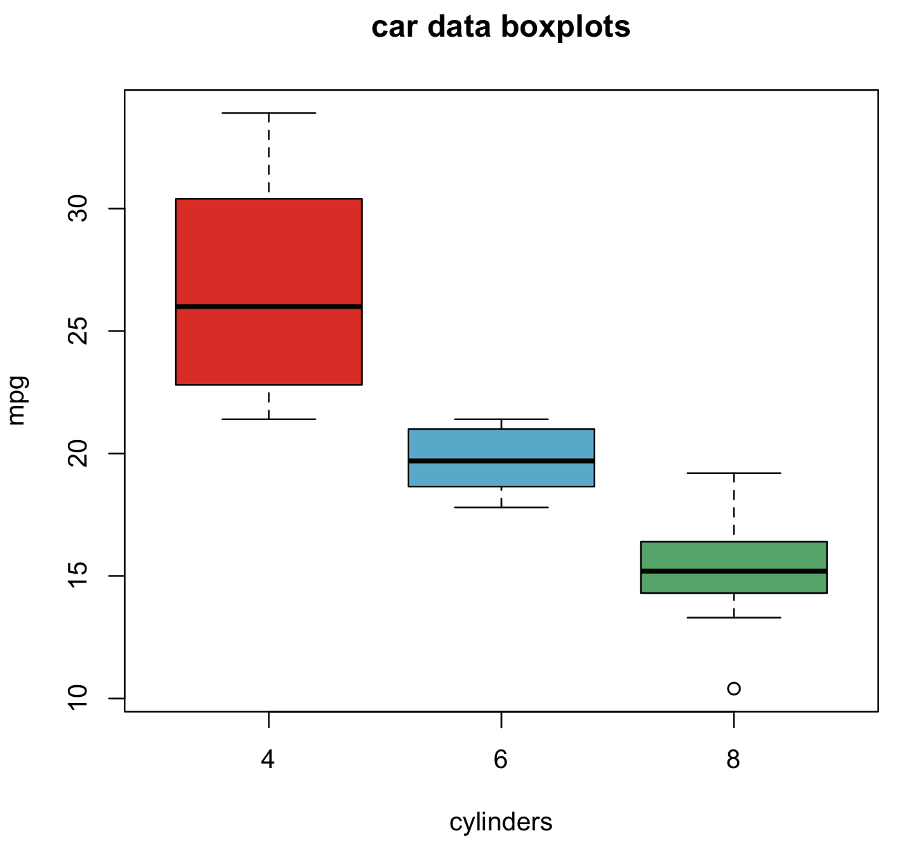
You can also visualize these summaries using boxplots for all variables using the R-package reshape2 and its function melt(). This will reshape the data frame to be more amenable for boxplots.
# you might need to install R-package 'reshape2'
install.packages("reshape2")
library(reshape2)
# reduce the "airway_data" to only the continuous variables.

airway_data_very_high_low <- airway_data
airway_data_reduced2 <- airway_data[,2:ncol(airway_data_very_high_low)]
head(airway_data_reduced2)
#  SRR1039508 SRR1039509 SRR1039512 SRR1039513 SRR1039516 SRR1039517 SRR1039520 SRR1039521
#1        723        486        904        445       1170       1097        806        604
#2          0          0          0          0          0          0          0          0
#3        467        523        616        371        582        781        417        509
#4        347        258        364        237        318        447        330        324
#5         96         81         73         66        118         94        102         74
#6          0          0          1          0          2          0          0          0
airway_data_reduced2_melted <- melt(airway_data_reduced2)
#No id variables; using all as measure variables
# we will change the names of the columns to reflect what they represent.
names(airway_data_reduced2_melted) <- c("sample", "expression")
head(airway_data_reduced2_melted)
#    sample expression
#1 SRR1039508   723
#2 SRR1039508     0
#3 SRR1039508   467
#4 SRR1039508   347
#5 SRR1039508    96
#6 SRR1039508     0

airway_data_reduced2_melted$expression <- log10(airway_data_reduced2_melted$expression + 1)
names(airway_data_reduced2_melted)[2] <- "log10_expression"
head(airway_data_reduced2_melted)
#      sample log10_expression
#1 SRR1039508         2.859739
#2 SRR1039508         0.000000
#3 SRR1039508         2.670246
#4 SRR1039508         2.541579
#5 SRR1039508         1.986772
#6 SRR1039508         0.000000


#airway_data boxplots using ggplot2

install.library("ggplot2")
library(ggplot2)

ggplot(airway_data_reduced2_melted, aes(x = sample, y = log10_expression, fill = sample)) +
                     geom_boxplot() +
                     stat_summary(fun = "mean", geom = "point", shape = 8, size = 2, color = "white")+
                     scale_y_continuous(breaks = c(0, 1, 2, 3, 4, 5), labels = c(1,10,100,1000,10000,100000)) +
labs(y = "log10 expression") 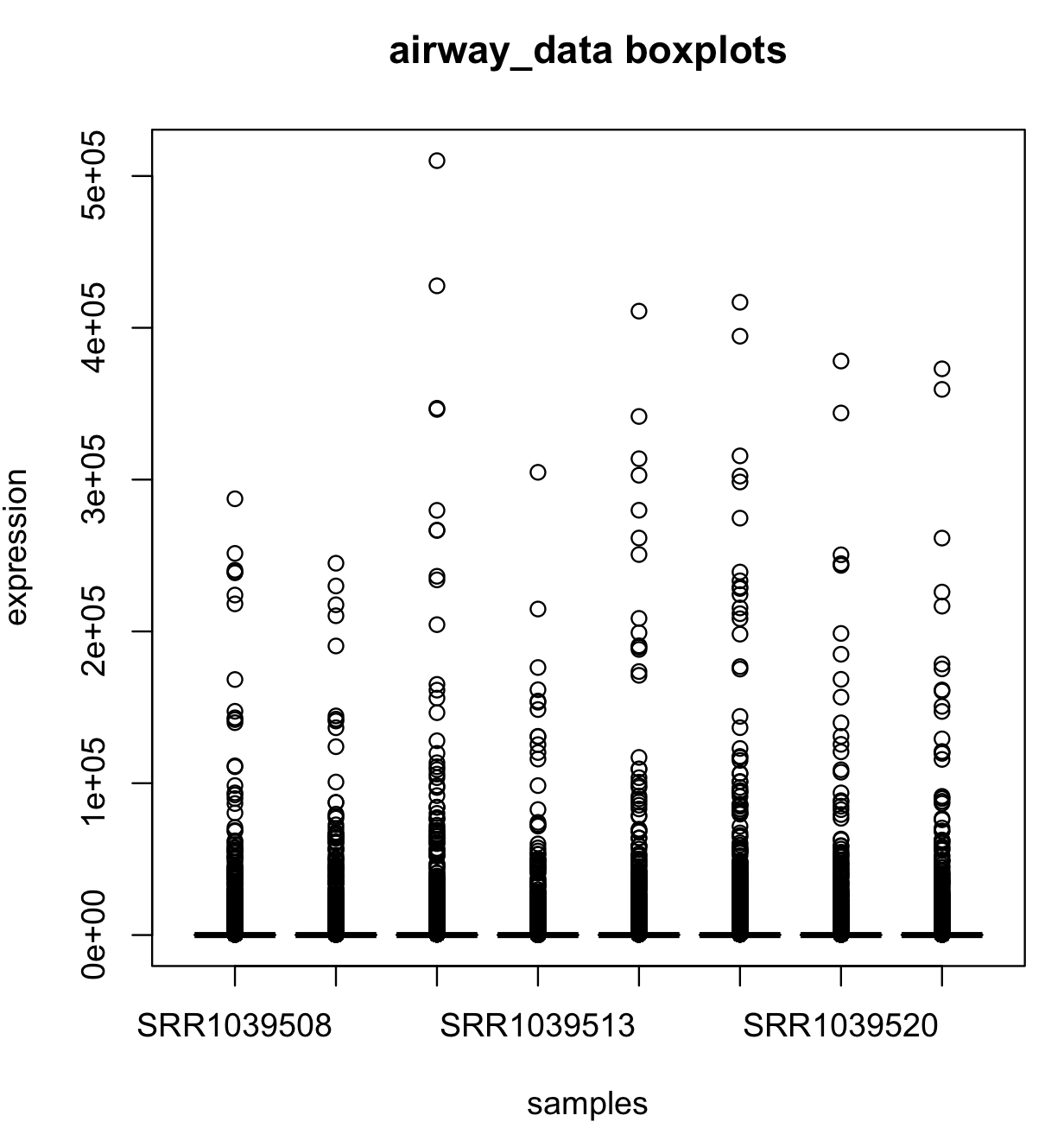
This figure is not very elegant (we will work with graph in that section). However, these boxplots are extremely skewed to low expression values.
3) We can discretize our data by creating groups based on criterium (e.g., threshold value). Such discrete groups can help us to define if a treatment or condition is reflected in our data or experimental groups. We will create a binary data frame for airway_data for the columns (variables) that represent the normalized gene expression for the samples that start withSRR. For this example, we will consider an arbitrary scale to divide into groups as: very high (x => 10000), high (10000 > x => 100) and low (x < 100) expression levels.
This task can be perform using a specialized R-package: purrr and its function modify() with a conditional ifelse(). We already introduce purrr on previous sessions. Notice that when we close some of the commands we use complex punctuation (i.e., (, ), {, }) and many mistakes can happen if you forget to close such punctuation pairs (i.e., missing one is a very common error)..
# we already installed R-package 'purrr'
library(purrr)
# we create an alternative object, so we original raw data airway_data
airway_data_very_high_low <- airway_data
# We will apply a the conditional
airway_data_very_high_low <- purrr::modify(airway_data_very_high_low,function(x) {ifelse(x >= 10000, "very_high",
                                                                                     ifelse( x >= 100, "high", "low"))})
head(airway_data_very_high_low)
#    ensgene SRR1039508 SRR1039509 SRR1039512 SRR1039513 SRR1039516 SRR1039517 SRR1039520 SRR1039521
#1 very_high       high       high       high       high       high       high       high       high
#2 very_high        low        low        low        low        low        low        low        low
#3 very_high       high       high       high       high       high       high       high       high
#4 very_high       high       high       high       high       high       high       high       high
#5 very_high        low        low        low        low       high        low       high        low
#6 very_high        low        low        low        low        low        low        low        low
#...
During the process above, we have “lost” the values of our variable ensgene that contains the names of the loci. We can add it back from our original data frame airway_data as indicated next.
airway_data_very_high_low$ensgene <- airway_data$ensgene
head(airway_data_very_high_low)
#          ensgene SRR1039508 SRR1039509 SRR1039512 SRR1039513 SRR1039516 SRR1039517 SRR1039520 SRR1039521
#1 ENSG00000000003       high       high       high       high       high       high       high       high
#2 ENSG00000000005        low        low        low        low        low        low        low        low
##3 ENSG00000000419       high       high       high       high       high       high       high       high
#4 ENSG00000000457       high       high       high       high       high       high       high       high
#5 ENSG00000000460        low        low        low        low       high        low       high        low
#6 ENSG00000000938        low        low        low        low        low        low        low        low
#...
4) With this discretized data frame airway_data_very_high_low, we can perform contingency tables. These are a type of table in a matrix format that displays the frequency distribution of the variables tested. We will exclude the first column ensgene because it has unique values.
airway_data_reduced <- airway_data_very_high_low[,2:ncol(airway_data_very_high_low)]
# collect frequencies on samples
summary_frequencies_airway_data <- list()
for(i in 1:ncol(airway_data_reduced)) {
                    sample_name <- names(airway_data_reduced[i])
                      one_table <- table(airway_data_reduced[i])
                      # from table to vector
          one_contigency_vector <- as.numeric(one_table)
                      # add names of categories
   names(one_contigency_vector) <- names(one_table)
                 one_data_frame <- as.data.frame(one_contigency_vector)
                     # add name of sample
          names(one_data_frame) <- sample_name
                     # collect results in list
    summary_frequencies_airway_data[[i]] <- one_data_frame
                                }
summary_frequencies_airway_data
#[[[1]]
#          SRR1039508
#high           11051
#low            27372
#very_high        271
#
#[[2]]
#          SRR1039509
#high           10708
#low            27722
#very_high        264
#...
With the list summary_frequencies_airway_data, we can cover it to a data frame by binding each vector as a column using two functions do.call() and cbind().
final_summary_all_samples_df <- do.call(cbind, summary_frequencies_airway_data)
final_summary_all_samples_df
#          SRR1039508 SRR1039509 SRR1039512 SRR1039513 SRR1039516 SRR1039517 SRR1039520 SRR1039521
#high           11051      10708      11268      10107      11203      11242      10946      10813
#low            27372      27722      27066      28402      27148      26961      27510      27595
#very_high        271        264        360        185        343        491        238        286
5) With this data frame, we can test these discretized variables for independence using a chi-squared test with the function summary().
For example, we can compare two of the airway_data_reduced samples (i.e., columns). Notice that I use a ; command at the end of one line of commands, this allows you to paste several commands next to each other as if they were in new lines.
sample_names <- names(airway_data_reduced)[1:2]
title_test <- paste0(sample_names, collapse ="..vs..")
contigency_result <- summary(table(airway_data_reduced[,1], airway_data_reduced[,2]))
cat(title_test, "\n"); print(contigency_result)
#SRR1039508..vs..SRR1039509
#Number of cases in table: 38694
#Number of factors: 2
#Test for independence of all factors:
#   Chisq = 58193, df = 4, p-value = 0
#   Chi-squared approximation may be incorrect
These results indicate that we can conclude that these samples are likely independent, but the large number of cases 38694 might have inflated the Chisq statistic.
Next we have an interesting loop for you to dissect, it will run all pairwise contingency tests, report the process, and add names of the pairs being compared. Notice the iterative variable counter and function break that breaks the loop when it has finished.
counter <- 0
collect_test_independence <- list()

for(i in 1:ncol(airway_data_reduced)) {
               # i <- 1
               names_sample_i <- names(airway_data_reduced)[i]
                n <- i + 1
      upper_limit <- ncol(airway_data_reduced)+1
                if(n < upper_limit) {
                    cat("sample:",names_sample_i, "..vs..")
                      for(j in n:ncol(airway_data_reduced)) {
                                    counter <- counter + 1
                                    names_sample_j <- names(airway_data_reduced)[j]
                                    cat(names_sample_j, "....")
                                  list_name <- paste0(names_sample_i,"..vs..", names_sample_j)
       collect_test_independence[[counter]] <- summary(table(airway_data_reduced[,i], airway_data_reduced[,j]))
  names(collect_test_independence)[counter] <- list_name
                                                             }
                                                           cat("\n")
                                   } else {break}
                                        }

#sample: SRR1039508 ..vs..SRR1039509 ....SRR1039512 ....SRR1039513 ....SRR1039516 ....SRR1039517 ....SRR1039520 ....SRR1039521 ....
#sample: SRR1039509 ..vs..SRR1039512 ....SRR1039513 ....SRR1039516 ....SRR1039517 ....SRR1039520 ....SRR1039521 ....
#sample: SRR1039512 ..vs..SRR1039513 ....SRR1039516 ....SRR1039517 ....SRR1039520 ....SRR1039521 ....
#sample: SRR1039513 ..vs..SRR1039516 ....SRR1039517 ....SRR1039520 ....SRR1039521 ....
#sample: SRR1039516 ..vs..SRR1039517 ....SRR1039520 ....SRR1039521 ....
#sample: SRR1039517 ..vs..SRR1039520 ....SRR1039521 ....
#sample: SRR1039520 ..vs..SRR1039521 ....

# if you call the collect_test_independence, you will get the statistics for independence
collect_test_independence
#$SRR1039508..vs..SRR1039509
#Number of cases in table: 38694
#Number of factors: 2
#Test for independence of all factors:
#   Chisq = 58193, df = 4, p-value = 0
#   Chi-squared approximation may be incorrect
#
#$SRR1039508..vs..SRR1039512
#Number of cases in table: 38694
#Number of factors: 2
#Test for independence of all factors:
#   Chisq = 58274, df = 4, p-value = 0
#   Chi-squared approximation may be incorrect
6.2 Sub-setting your dataset
It is often the case that you do not want to run some analysis with some part and not all your data. This will require that your subset (i.e., select some parts) your data.
We will explore some different forms to subset your data. For that purpose, we will use Cars93 dataset from the R-package MASS.
## we can install MASS and load the dataset for this example
install.packages("MASS")
library(MASS)
## We assign Cars93 dataset to an object
my_cars <- Cars93
str(my_cars)
#'data.frame':  93 obs. of  27 variables:
# $ Manufacturer      : Factor w/ 32 levels "Acura","Audi",..: 1 1 2 2 3 4 4 4 4 5 ...
# $ Model             : Factor w/ 93 levels "100","190E","240",..: 49 56 9 1 6 24 54 74 73 35 ...
# $ Type              : Factor w/ 6 levels "Compact","Large",..: 4 3 1 3 3 3 2 2 3 2 ...
# $ Min.Price         : num  12.9 29.2 25.9 30.8 23.7 14.2 19.9 22.6 26.3 33 ...
# $ Price             : num  15.9 33.9 29.1 37.7 30 15.7 20.8 23.7 26.3 34.7 ...
# $ Max.Price         : num  18.8 38.7 32.3 44.6 36.2 17.3 21.7 24.9 26.3 36.3 ...
# $ MPG.city          : int  25 18 20 19 22 22 19 16 19 16 ...
# $ MPG.highway       : int  31 25 26 26 30 31 28 25 27 25 ...
# $ AirBags           : Factor w/ 3 levels "Driver & Passenger",..: 3 1 2 1 2 2 2 2 2 2 ...
# $ DriveTrain        : Factor w/ 3 levels "4WD","Front",..: 2 2 2 2 3 2 2 3 2 2 ...
# $ Cylinders         : Factor w/ 6 levels "3","4","5","6",..: 2 4 4 4 2 2 4 4 4 5 ...
# $ EngineSize        : num  1.8 3.2 2.8 2.8 3.5 2.2 3.8 5.7 3.8 4.9 ...
# $ Horsepower        : int  140 200 172 172 208 110 170 180 170 200 ...
# $ RPM               : int  6300 5500 5500 5500 5700 5200 4800 4000 4800 4100 ...
# $ Rev.per.mile      : int  2890 2335 2280 2535 2545 2565 1570 1320 1690 1510 ...
# $ Man.trans.avail   : Factor w/ 2 levels "No","Yes": 2 2 2 2 2 1 1 1 1 1 ...
# $ Fuel.tank.capacity: num  13.2 18 16.9 21.1 21.1 16.4 18 23 18.8 18 ...
# $ Passengers        : int  5 5 5 6 4 6 6 6 5 6 ...
# $ Length            : int  177 195 180 193 186 189 200 216 198 206 ...
# $ Wheelbase         : int  102 115 102 106 109 105 111 116 108 114 ...
# $ Width             : int  68 71 67 70 69 69 74 78 73 73 ...
# $ Turn.circle       : int  37 38 37 37 39 41 42 45 41 43 ...
# $ Rear.seat.room    : num  26.5 30 28 31 27 28 30.5 30.5 26.5 35 ...
# $ Luggage.room      : int  11 15 14 17 13 16 17 21 14 18 ...
# $ Weight            : int  2705 3560 3375 3405 3640 2880 3470 4105 3495 3620 ...
# $ Origin            : Factor w/ 2 levels "USA","non-USA": 2 2 2 2 2 1 1 1 1 1 ...
# $ Make              : Factor w/ 93 levels "Acura Integra",..: 1 2 4 3 5 6 7 9 8 10 ...
For example, you might want to include only some variables. We will select Origin, Manufacturer,Price, Passengers, MPG.city, and EngineSize.
For that purpose, we use the function subset() and notice it syntax.
subset_my_cars <- subset(my_cars, select = c(Origin, Manufacturer, Price, Passengers, MPG.city, EngineSize))
head(subset_my_cars)
#  Origin Manufacturer Price Passengers MPG.city EngineSize
#1 non-USA        Acura  15.9          5       25        1.8
#2 non-USA        Acura  33.9          5       18        3.2
#3 non-USA         Audi  29.1          5       20        2.8
#4 non-USA         Audi  37.7          6       19        2.8
#5 non-USA          BMW  30.0          4       22        3.5
#6     USA        Buick  15.7          6       22        2.2
You might want to include groups based on a character name (i.e., equal to some term). We will select only cars with Origin from the USA.
only_usa_subset_my_cars <- subset(subset_my_cars, Origin == "USA")
head(only_usa_subset_my_cars)
#   Origin Manufacturer Price Passengers MPG.city EngineSize
#6     USA        Buick  15.7          6       22        2.2
#7     USA        Buick  20.8          6       19        3.8
#8     USA        Buick  23.7          6       16        5.7
#9     USA        Buick  26.3          5       19        3.8
#10    USA     Cadillac  34.7          6       16        4.9
#11    USA     Cadillac  40.1          5       16        4.6
You might want to include groups based on a value. We will select only cars with an EngineSize more or equal to 3.
only_large_engine_subset_my_cars <- subset(subset_my_cars, EngineSize >= 3.0)
head(only_large_engine_subset_my_cars)
#       Origin Manufacturer Price Passengers MPG.city EngineSize
#2  non-USA        Acura  33.9          5       18        3.2
#5  non-USA          BMW  30.0          4       22        3.5
#7      USA        Buick  20.8          6       19        3.8
#8      USA        Buick  23.7          6       16        5.7
#9      USA        Buick  26.3          5       19        3.8
#10     USA     Cadillac  34.7          6       16        4.9
You might want to combine several considerations. We will select only cars not made in the USA with an EngineSize less or equal to 4.
some_of_my_cars <- subset(subset_my_cars, Origin == "non-USA" & EngineSize <= 4.0)
head(some_of_my_cars)
#    Origin Manufacturer Price Passengers MPG.city EngineSize
#1  non-USA        Acura  15.9          5       25        1.8
#2  non-USA        Acura  33.9          5       18        3.2
#3  non-USA         Audi  29.1          5       20        2.8
#4  non-USA         Audi  37.7          6       19        2.8
#5  non-USA          BMW  30.0          4       22        3.5
#39 non-USA          Geo   8.4          4       46        1.0
6.3 Transposing (rotating) your dataset
Some datasets might have the “wrong” orientation (e.g., individuals as columns and variables as rows). This usually depends on the source data and for most purposes, you migth want your individuals as rows and each column with the variable measurements. We can correct this “wrong” orientation by transposing your data frame or matrix.
Here is an example using deaths dataset from the R-package MASS. This is a time series giving the monthly deaths from bronchitis, emphysema and asthma in the UK, 1974-1979, both sexes (deaths). I retyped the data into a data frame to make it easy to transpose (rotate) this dataset.
## this is time series dataset as a data frame
UK_deaths <- data.frame(year_1974=c(3035,2552,2704,2554,2014,1655,1721,1524,1596,2074,2199,2512),
                        year_1975 = c(2933,2889,2938,2497,1870,1726,1607,1545,1396,1787,2076,2837),
                        year_1976 = c(2787,3891,3179,2011,1636,1580,1489,1300,1356,1653,2013,2823),
                        year_1977 = c(3102,2294,2385,2444,1748,1554,1498,1361,1346,1564,1640,2293),
                        year_1978 = c(2815,3137,2679,1969,1870,1633,1529,1366,1357,1570,1535,2491),
                        year_1979 = c(3084,2605,2573,2143,1693,1504,1461,1354,1333,1492,1781,1915), stringsAsFactors = FALSE)
rownames(UK_deaths) <- c("Jan","Feb","Mar","Apr","May","Jun","Jul","Aug","Sep","Oct","Nov","Dec")

## this dataset has months as rows and years as columns

UK_deaths
#    year_1974 year_1975 year_1976 year_1977 year_1978 year_1979
# Jan      3035      2933      2787      3102      2815      3084
# Feb      2552      2889      3891      2294      3137      2605
# Mar      2704      2938      3179      2385      2679      2573
# Apr      2554      2497      2011      2444      1969      2143
# May      2014      1870      1636      1748      1870      1693
# Jun      1655      1726      1580      1554      1633      1504
# Jul      1721      1607      1489      1498      1529      1461
# Aug      1524      1545      1300      1361      1366      1354
# Sep      1596      1396      1356      1346      1357      1333
# Oct      2074      1787      1653      1564      1570      1492
# Nov      2199      2076      2013      1640      1535      1781
# Dec      2512      2837      2823      2293      2491      1915
str(UK_deaths)
#'data.frame':  12 obs. of  6 variables:
# $ year_1974: num  3035 2552 2704 2554 2014 ...
# $ year_1975: num  2933 2889 2938 2497 1870 ...
# $ year_1976: num  2787 3891 3179 2011 1636 ...
# $ year_1977: num  3102 2294 2385 2444 1748 ...
# $ year_1978: num  2815 3137 2679 1969 1870 ...
# $ year_1979: num  3084 2605 2573 2143 1693 ..

## we can transpose this UK_deaths to have months as columns
UK_deaths_t <- as.data.frame(t(UK_deaths),stringsAsFactors = FALSE)
class(UK_deaths_t)
#[1] "data.frame"

UK_deaths_t
#           Jan  Feb  Mar  Apr  May  Jun  Jul  Aug  Sep  Oct  Nov  Dec
# year_1974 3035 2552 2704 2554 2014 1655 1721 1524 1596 2074 2199 2512
# year_1975 2933 2889 2938 2497 1870 1726 1607 1545 1396 1787 2076 2837
# year_1976 2787 3891 3179 2011 1636 1580 1489 1300 1356 1653 2013 2823
# year_1977 3102 2294 2385 2444 1748 1554 1498 1361 1346 1564 1640 2293
# year_1978 2815 3137 2679 1969 1870 1633 1529 1366 1357 1570 1535 2491
# year_1979 3084 2605 2573 2143 1693 1504 1461 1354 1333 1492 1781 1915
6.4 Dealing with missing (NA) values
Most datasets would have some missing values usually coded as NA, <NaN or
We will work with some build and complete datasets. Then, we will introduce missing values.
## the mtcars is comparisons between 32 automobiles (1973–74 models)
my_mtcars <- mtcars
my_mtcars$car_name <- rownames(my_mtcars)
rownames(my_mtcars) <- NULL
my_mtcars
#    mpg cyl  disp  hp drat    wt  qsec vs am gear carb            car_name
# 1  21.0   6 160.0 110 3.90 2.620 16.46  0  1    4    4           Mazda RX4
# 2  21.0   6 160.0 110 3.90 2.875 17.02  0  1    4    4       Mazda RX4 Wag
# 3  22.8   4 108.0  93 3.85 2.320 18.61  1  1    4    1          Datsun 710
# 4  21.4   6 258.0 110 3.08 3.215 19.44  1  0    3    1      Hornet 4 Drive
# 5  18.7   8 360.0 175 3.15 3.440 17.02  0  0    3    2   Hornet Sportabout
# 6  18.1   6 225.0 105 2.76 3.460 20.22  1  0    3    1             Valiant
# 7  14.3   8 360.0 245 3.21 3.570 15.84  0  0    3    4          Duster 360
# 8  24.4   4 146.7  62 3.69 3.190 20.00  1  0    4    2           Merc 240D
# 9  22.8   4 140.8  95 3.92 3.150 22.90  1  0    4    2            Merc 230
# 10 19.2   6 167.6 123 3.92 3.440 18.30  1  0    4    4            Merc 280
# 11 17.8   6 167.6 123 3.92 3.440 18.90  1  0    4    4           Merc 280C
# 12 16.4   8 275.8 180 3.07 4.070 17.40  0  0    3    3          Merc 450SE
# 13 17.3   8 275.8 180 3.07 3.730 17.60  0  0    3    3          Merc 450SL
# 14 15.2   8 275.8 180 3.07 3.780 18.00  0  0    3    3         Merc 450SLC
# 15 10.4   8 472.0 205 2.93 5.250 17.98  0  0    3    4  Cadillac Fleetwood
# 16 10.4   8 460.0 215 3.00 5.424 17.82  0  0    3    4 Lincoln Continental
# 17 14.7   8 440.0 230 3.23 5.345 17.42  0  0    3    4   Chrysler Imperial
# 18 32.4   4  78.7  66 4.08 2.200 19.47  1  1    4    1            Fiat 128
# 19 30.4   4  75.7  52 4.93 1.615 18.52  1  1    4    2         Honda Civic
# 20 33.9   4  71.1  65 4.22 1.835 19.90  1  1    4    1      Toyota Corolla
# 21 21.5   4 120.1  97 3.70 2.465 20.01  1  0    3    1       Toyota Corona
# 22 15.5   8 318.0 150 2.76 3.520 16.87  0  0    3    2    Dodge Challenger
# 23 15.2   8 304.0 150 3.15 3.435 17.30  0  0    3    2         AMC Javelin
# 24 13.3   8 350.0 245 3.73 3.840 15.41  0  0    3    4          Camaro Z28
# 25 19.2   8 400.0 175 3.08 3.845 17.05  0  0    3    2    Pontiac Firebird
# 26 27.3   4  79.0  66 4.08 1.935 18.90  1  1    4    1           Fiat X1-9
# 27 26.0   4 120.3  91 4.43 2.140 16.70  0  1    5    2       Porsche 914-2
# 28 30.4   4  95.1 113 3.77 1.513 16.90  1  1    5    2        Lotus Europa
# 29 15.8   8 351.0 264 4.22 3.170 14.50  0  1    5    4      Ford Pantera L
# 30 19.7   6 145.0 175 3.62 2.770 15.50  0  1    5    6        Ferrari Dino
# 31 15.0   8 301.0 335 3.54 3.570 14.60  0  1    5    8       Maserati Bora
# 32 21.4   4 121.0 109 4.11 2.780 18.60  1  1    4    2          Volvo 142E

## Lets introduce some NA values randomly
my_mtcars_with_NA <- as.data.frame(lapply(my_mtcars, function(x_df) x_df[ sample(c(TRUE, NA), prob = c(0.85, 0.15), size = length(x_df), replace = TRUE) ]))
my_mtcars_with_NA
#    mpg cyl  disp  hp drat    wt  qsec vs am gear carb            car_name
# 1  21.0   6 160.0 110 3.90 2.620 16.46  0  1    4    4                <NA>
# 2  21.0   6 160.0  NA 3.90 2.875 17.02  0 NA    4   NA                <NA>
# 3  22.8   4 108.0  93 3.85 2.320    NA NA  1    4    1          Datsun 710
# 4    NA   6 258.0 110 3.08 3.215    NA  1  0    3    1      Hornet 4 Drive
# 5  18.7   8 360.0 175 3.15 3.440 17.02  0  0    3    2   Hornet Sportabout
# 6  18.1   6 225.0 105 2.76 3.460 20.22  1 NA    3   NA             Valiant
# 7  14.3   8 360.0  NA 3.21 3.570    NA  0  0    3   NA          Duster 360
# 8  24.4   4 146.7  62   NA 3.190 20.00  1  0    4    2           Merc 240D
# 9  22.8   4    NA  95   NA 3.150 22.90  1  0    4   NA            Merc 230
# 10 19.2   6 167.6 123 3.92 3.440 18.30  1  0   NA   NA                <NA>
# 11 17.8   6 167.6 123 3.92 3.440 18.90  1  0    4   NA           Merc 280C
# 12 16.4   8 275.8  NA 3.07 4.070 17.40  0  0    3    3          Merc 450SE
# 13 17.3   8 275.8 180 3.07 3.730 17.60  0  0    3    3          Merc 450SL
# 14 15.2   8    NA 180 3.07 3.780    NA  0  0    3    3                <NA>
# 15 10.4  NA 472.0 205 2.93    NA 17.98  0  0    3    4  Cadillac Fleetwood
# 16 10.4  NA 460.0 215 3.00 5.424 17.82  0 NA    3    4 Lincoln Continental
# 17 14.7   8 440.0  NA 3.23 5.345    NA  0  0    3    4   Chrysler Imperial
# 18 32.4   4  78.7  66   NA 2.200 19.47  1  1   NA    1            Fiat 128
# 19 30.4   4  75.7  52 4.93 1.615 18.52  1  1    4    2         Honda Civic
# 20 33.9   4  71.1  NA 4.22 1.835 19.90 NA NA    4    1      Toyota Corolla
# 21 21.5   4 120.1  97 3.70 2.465 20.01  1  0    3    1       Toyota Corona
# 22 15.5   8 318.0 150 2.76 3.520 16.87  0  0    3    2                <NA>
# 23 15.2   8    NA 150 3.15    NA 17.30  0  0    3    2         AMC Javelin
# 24   NA   8    NA 245 3.73    NA 15.41  0 NA    3    4          Camaro Z28
# 25   NA   8 400.0 175   NA 3.845 17.05  0  0    3    2    Pontiac Firebird
# 26   NA   4  79.0  66 4.08 1.935 18.90  1  1   NA    1           Fiat X1-9
# 27 26.0   4 120.3  91 4.43    NA 16.70  0 NA    5   NA       Porsche 914-2
# 28 30.4   4  95.1 113 3.77 1.513 16.90  1  1    5   NA        Lotus Europa
# 29 15.8   8 351.0 264 4.22 3.170 14.50  0  1    5    4      Ford Pantera L
# 30   NA   6 145.0 175 3.62    NA 15.50  0  1    5    6                <NA>
# 31 15.0   8 301.0 335 3.54 3.570 14.60  0  1    5    8       Maserati Bora
# 32 21.4   4 121.0 109 4.11 2.780 18.60  1  1   NA   NA          Volvo 142E
You can compare these two datasets and notice several cells with values as NA (if variable is numeric) and
We can remove all rows with at least one NA value using the function complete.cases().
## remove all rows with at least on NA
my_mtcars_complete_rows <- my_mtcars_with_NA[complete.cases(my_mtcars_with_NA), ]
my_mtcars_complete_rows
#     mpg cyl  disp  hp drat    wt  qsec vs am gear carb          car_name
# 5  18.7   8 360.0 175 3.15 3.440 17.02  0  0    3    2 Hornet Sportabout
# 13 17.3   8 275.8 180 3.07 3.730 17.60  0  0    3    3        Merc 450SL
# 19 30.4   4  75.7  52 4.93 1.615 18.52  1  1    4    2       Honda Civic
# 21 21.5   4 120.1  97 3.70 2.465 20.01  1  0    3    1     Toyota Corona
# 29 15.8   8 351.0 264 4.22 3.170 14.50  0  1    5    4    Ford Pantera L
# 31 15.0   8 301.0 335 3.54 3.570 14.60  0  1    5    8     Maserati Bora
We can remove rows with at least one NA value on specific columns using the function complete.cases().
## remove rows with at least one NA in columns "mpg" and "cyl"
my_mtcars_complete_rows_mpg_cyl <- my_mtcars_with_NA[complete.cases(my_mtcars_with_NA[,c("mpg","cyl")]), ]
my_mtcars_complete_rows_mpg_cyl
#    mpg cyl  disp  hp drat    wt  qsec vs am gear carb          car_name
# 1  21.0   6 160.0 110 3.90 2.620 16.46  0  1    4    4              <NA>
# 2  21.0   6 160.0  NA 3.90 2.875 17.02  0 NA    4   NA              <NA>
# 3  22.8   4 108.0  93 3.85 2.320    NA NA  1    4    1        Datsun 710
# 5  18.7   8 360.0 175 3.15 3.440 17.02  0  0    3    2 Hornet Sportabout
# 6  18.1   6 225.0 105 2.76 3.460 20.22  1 NA    3   NA           Valiant
# 7  14.3   8 360.0  NA 3.21 3.570    NA  0  0    3   NA        Duster 360
# 8  24.4   4 146.7  62   NA 3.190 20.00  1  0    4    2         Merc 240D
# 9  22.8   4    NA  95   NA 3.150 22.90  1  0    4   NA          Merc 230
# 10 19.2   6 167.6 123 3.92 3.440 18.30  1  0   NA   NA              <NA>
# 11 17.8   6 167.6 123 3.92 3.440 18.90  1  0    4   NA         Merc 280C
# 12 16.4   8 275.8  NA 3.07 4.070 17.40  0  0    3    3        Merc 450SE
# 13 17.3   8 275.8 180 3.07 3.730 17.60  0  0    3    3        Merc 450SL
# 14 15.2   8    NA 180 3.07 3.780    NA  0  0    3    3              <NA>
# 17 14.7   8 440.0  NA 3.23 5.345    NA  0  0    3    4 Chrysler Imperial
# 18 32.4   4  78.7  66   NA 2.200 19.47  1  1   NA    1          Fiat 128
# 19 30.4   4  75.7  52 4.93 1.615 18.52  1  1    4    2       Honda Civic
# 20 33.9   4  71.1  NA 4.22 1.835 19.90 NA NA    4    1    Toyota Corolla
# 21 21.5   4 120.1  97 3.70 2.465 20.01  1  0    3    1     Toyota Corona
# 22 15.5   8 318.0 150 2.76 3.520 16.87  0  0    3    2              <NA>
# 23 15.2   8    NA 150 3.15    NA 17.30  0  0    3    2       AMC Javelin
# 27 26.0   4 120.3  91 4.43    NA 16.70  0 NA    5   NA     Porsche 914-2
# 28 30.4   4  95.1 113 3.77 1.513 16.90  1  1    5   NA      Lotus Europa
# 29 15.8   8 351.0 264 4.22 3.170 14.50  0  1    5    4    Ford Pantera L
# 31 15.0   8 301.0 335 3.54 3.570 14.60  0  1    5    8     Maserati Bora
# 32 21.4   4 121.0 109 4.11 2.780 18.60  1  1   NA   NA        Volvo 142E
Notice that columns called mpg and cyl have complete values a no missing NA.
You can also replace NA for specific values, for example as zero (0).
## lets get the am variable as a vector
my_NA_am_variable <- my_mtcars_with_NA$am
my_NA_am_variable
#[1] 1 NA 1 0 NA 0 0 0 0 0 0 0 0 0 0 0 0 1 1 NA 0 0 0 0 0 1 1 NA 1 1 1 1

## lets replace NA in the variable am for 0
my_replaced_am_variable <- ifelse(is.na(my_NA_am_variable),0,my_NA_am_variable)
my_replaced_am_variable
# [1] 1 0 1 0 0 0 0 0 0 0 0 0 0 0 0 0 0 1 1 0 0 0 0 0 0 1 1 0 1 1 1 1

## lets put back the compled am variable in our data frame
my_mtcars_with_completed_am <- my_mtcars_with_NA
my_mtcars_with_completed_am$am <- my_replaced_am_variable
my_mtcars_with_completed_am
#    mpg cyl  disp  hp drat    wt  qsec vs am gear carb            car_name
# 1  21.0   6 160.0 110 3.90 2.620 16.46  0  1    4    4                <NA>
# 2  21.0   6 160.0  NA 3.90 2.875 17.02  0  0    4   NA                <NA>
# 3  22.8   4 108.0  93 3.85 2.320    NA NA  1    4    1          Datsun 710
# 4    NA   6 258.0 110 3.08 3.215    NA  1  0    3    1      Hornet 4 Drive
# 5  18.7   8 360.0 175 3.15 3.440 17.02  0  0    3    2   Hornet Sportabout
# 6  18.1   6 225.0 105 2.76 3.460 20.22  1  0   3   NA             Valiant
# 7  14.3   8 360.0  NA 3.21 3.570    NA  0  0    3   NA          Duster 360
# 8  24.4   4 146.7  62   NA 3.190 20.00  1  0    4    2           Merc 240D
# 9  22.8   4    NA  95   NA 3.150 22.90  1  0    4   NA            Merc 230
# 10 19.2   6 167.6 123 3.92 3.440 18.30  1  0   NA   NA                <NA>
# 11 17.8   6 167.6 123 3.92 3.440 18.90  1  0    4   NA           Merc 280C
# 12 16.4   8 275.8  NA 3.07 4.070 17.40  0  0    3    3          Merc 450SE
# 13 17.3   8 275.8 180 3.07 3.730 17.60  0  0    3    3          Merc 450SL
# 14 15.2   8    NA 180 3.07 3.780    NA  0  0    3    3                <NA>
# 15 10.4  NA 472.0 205 2.93    NA 17.98  0  0    3    4  Cadillac Fleetwood
# 16 10.4  NA 460.0 215 3.00 5.424 17.82  0  0    3    4 Lincoln Continental
# 17 14.7   8 440.0  NA 3.23 5.345    NA  0  0    3    4   Chrysler Imperial
# 18 32.4   4  78.7  66   NA 2.200 19.47  1  1   NA    1            Fiat 128
# 19 30.4   4  75.7  52 4.93 1.615 18.52  1  1    4    2         Honda Civic
# 20 33.9   4  71.1  NA 4.22 1.835 19.90 NA  0    4    1      Toyota Corolla
# 21 21.5   4 120.1  97 3.70 2.465 20.01  1  0    3    1       Toyota Corona
# 22 15.5   8 318.0 150 2.76 3.520 16.87  0  0    3    2                <NA>
# 23 15.2   8    NA 150 3.15    NA 17.30  0  0    3    2         AMC Javelin
# 24   NA   8    NA 245 3.73    NA 15.41  0  0   3    4          Camaro Z28
# 25   NA   8 400.0 175   NA 3.845 17.05  0  0    3    2    Pontiac Firebird
# 26   NA   4  79.0  66 4.08 1.935 18.90  1  1   NA    1           Fiat X1-9
# 27 26.0   4 120.3  91 4.43    NA 16.70  0  0    5   NA       Porsche 914-2
# 28 30.4   4  95.1 113 3.77 1.513 16.90  1  1    5   NA        Lotus Europa
# 29 15.8   8 351.0 264 4.22 3.170 14.50  0  1    5    4      Ford Pantera L
# 30   NA   6 145.0 175 3.62    NA 15.50  0  1    5    6                <NA>
# 31 15.0   8 301.0 335 3.54 3.570 14.60  0  1    5    8       Maserati Bora
# 32 21.4   4 121.0 109 4.11 2.780 18.60  1  1   NA   NA          Volvo 142E
Notice that columns called am is now complete with no missing NA.
In some tests or statistics, you can explicitly exclude NA in the calculations using na.rm = TRUE.
## Lets get the mean value of mpg without removing NAs.
mean(my_mtcars_with_NA$mpg)
#[1] NA

## we get an NA and a warning. Now, lets repat with the na.rm = TRUE
mean(my_mtcars_with_NA$mpg,na.rm = TRUE)
#[1] 20.07407
You can get the mean of all columns in the data frame.
## We need to remove the discrete variable car_name
my_mtcars_with_NA_2 <- subset(my_mtcars_with_NA, select = !names(my_mtcars_with_NA) %in% "car_name")
head(my_mtcars_with_NA_2)
#   mpg cyl disp  hp drat    wt  qsec vs am gear carb
# 1 21.0   6  160 110 3.90 2.620 16.46  0  1    4    4
# 2 21.0   6  160  NA 3.90 2.875 17.02  0 NA    4   NA
# 3 22.8   4  108  93 3.85 2.320    NA NA  1    4    1
# 4   NA   6  258 110 3.08 3.215    NA  1  0    3    1
# 5 18.7   8  360 175 3.15 3.440 17.02  0  0    3    2
# 6 18.1   6  225 105 2.76 3.460 20.22  1 NA    3   NA

## We try to get the mean of all columns and fail
colMeans(my_mtcars_with_NA_2)
# mpg  cyl disp   hp drat   wt qsec   vs   am gear carb
#   NA   NA   NA   NA   NA   NA   NA   NA   NA   NA   NA

## We try now by removing NA
colMeans(my_mtcars_with_NA_2,na.rm = TRUE)
#       mpg         cyl        disp          hp        drat          wt        qsec          vs          am        gear        carb
# 20.0740741   6.0666667 225.4464286 143.1111111   3.5828571   3.1672963  17.8462963   0.4000000   0.3846154   3.6428571   2.8260870
You can do pair t.test() with cars with three classes of cylinders 4 and 6 with values on column mpg
## group of cars with 4 cylinders
mpg_4 <- subset(my_mtcars_with_NA, cyl == 4, select = mpg)
mpg_4
#     mpg
#3  22.8
#8  24.4
#9  22.8
#18 32.4
#19 30.4
#20 33.9
#21 21.5
#26   NA
#27 26.0
#28 30.4
#32 21.4

## group of cars with 6 cylinders
mpg_6 <- subset(my_mtcars_with_NA, cyl == 6, select = mpg)
mpg_6
#    mpg
#1  21.0
#2  21.0
#4    NA
#6  18.1
#10 19.2
#11 17.8
#30   NA

## We try to do a t.test for pair of groups
t.test(mpg_4, mpg_6, paired = FALSE)
#   Welch Two Sample t-test
#
#data:  mpg_4 and mpg_6
#t = 4.3493, df = 11.974, p-value = 0.0009507
#alternative hypothesis: true difference in means is not equal to 0
#95 percent confidence interval:
#  3.582259 10.777741
#sample estimates:
#mean of x mean of y
#    26.60     19.42
However, we try a similar wilcox.test() but we fail
## We try the wilcox.test and fail
wilcox.test(mpg_4, mpg_6, paired = FALSE)
# Error in wilcox.test.default(mpg_4, mpg_6, paired = FALSE) :
#  'x' must be numeric

## We need to remove NA
mpg_4_c <- mpg_4[complete.cases(mpg_4),]
mpg_4_c
#[1] 22.8 24.4 22.8 32.4 30.4 33.9 21.5 26.0 30.4 21.4
mpg_6_c <- mpg_6[complete.cases(mpg_6),]
mpg_6_c
#[1] 21.0 21.0 18.1 19.2 17.8

## We can try now again the wilcox.test
wilcox.test(mpg_4_c, mpg_6_c, paired = FALSE,)
#   Wilcoxon rank sum test with continuity correction
#
# data:  mpg_4_c and mpg_6_c
# W = 50, p-value = 0.002624
# alternative hypothesis: true location shift is not equal to 0
6.5 About p-values
In most of your statistical tests, you will pay attention to the number associated to a p-value. The general interpretation of p-values is that they represent the probability of getting results similar or as extreme as those for the null hypothesis assuming that this one is correct (e.g., an expected mean value or similar mean values between two groups assuming that they are from the same population). Likewise, p-values measure the probability that an observed differences between groups could have occurred just by random chance.
6.6 How to read p-values
In most cases, small or tiny p-value are of interest as they represent stronger evidence to reject the null hypothesis and opens the possibly for an alternative hypothesis or explanation. In practice, the significance level is stated by the researcher and in advance (e.g., p <0.05 is significant). The research then determines if the observed p-value is safe to reject the null hypothesis. In contrast, a p-value greater than 0.05 means that results do not deviate enough from those expected if the null hypothesis is true and these p-values are considered to be not statistically significant and fail to reject the null hypothesis.
To explore this further, we will use the mtcars dataset.
## the mtcars is comparisons between 32 automobiles (1973–74 models)
my_mtcars <- mtcars
my_mtcars$car_name <- rownames(my_mtcars)
rownames(my_mtcars) <- NULL
str(my_mtcars)
#'data.frame':  32 obs. of  12 variables:
# $ mpg     : num  21 21 22.8 21.4 18.7 18.1 14.3 24.4 22.8 19.2 ...
# $ cyl     : num  6 6 4 6 8 6 8 4 4 6 ...
# $ disp    : num  160 160 108 258 360 ...
# $ hp      : num  110 110 93 110 175 105 245 62 95 123 ...
# $ drat    : num  3.9 3.9 3.85 3.08 3.15 2.76 3.21 3.69 3.92 3.92 ...
# $ wt      : num  2.62 2.88 2.32 3.21 3.44 ...
# $ qsec    : num  16.5 17 18.6 19.4 17 ...
# $ vs      : num  0 0 1 1 0 1 0 1 1 1 ...
# $ am      : num  1 1 1 0 0 0 0 0 0 0 ...
# $ gear    : num  4 4 4 3 3 3 3 4 4 4 ...
# $ carb    : num  4 4 1 1 2 1 4 2 2 4 ...
# $ car_name: chr  "Mazda RX4" "Mazda RX4 Wag" "Datsun 710" "Hornet 4 Drive" ...

## group of cars with 4 cylinders
mpg_4 <- subset(my_mtcars, cyl == 4, select = mpg)

## group of 6 cylinders
mpg_6 <- subset(my_mtcars, cyl == 6, select = mpg)

## We try to do a t.test for pair of groups
t.test(mpg_4, mpg_6, paired = FALSE)
#   Welch Two Sample t-test
#
# data:  mpg_4 and mpg_6
# t = 4.7191, df = 12.956, p-value = 0.0004048
# alternative hypothesis: true difference in means is not equal to 0
# 95 percent confidence interval:
#  3.751376 10.090182
# sample estimates:
# mean of x mean of y
#  26.66364  19.74286
In this exercise, what does a p-value = 0.0004048 mean? This value indicates that if the null hypothesis tested were indeed true (i.e., the mean mpg for cars with 4 and 6 cylinders is equal), there would be a 4.048 in 10,000 chance of observing results at least as extreme were both groups will have the same mpg. This leads the researcher to reject the null hypothesis because either an extreme rare data result has been observed, or the null hypothesis is likely to be incorrect.
6.7 Multiple testing corrections
Consider that in many instances, we can perform multiple tests and obtain a collection of p-values. We can apply a multiple testing correction to adjust p-values obtained to correct for occurrence of false positives. These false positives are significant p-values that should be considered not informative and due by chance (i.e., you could do 100 tests, and some might be significant just by the larger number of tests performed).
In bioinformatics, it is common to perform hundreds of statistical testes (e.g., t-tests or ANOVAs) when you are comparing genetic results such as to find differentially expressed genes between a control and an experimental (study) group after the application of a treatment. The incidence of these genes falsely called as differentially expressed is proportional to the number of tests performed and the threshold p-value for significance (critical significance level).
We can illustrate this by assuming that we perform a t-test between two groups using the results derived from comparisons of gene expression between both. In this case, the probability by which the tests will be considered significantly (i.e., evidence of differential gene expression) is expressed by the p-value. We could use the standard threshold of p-value = 0.05, which signifies we have a 5% probability to find a significant differentially expressed gene by chance alone (i.e., not the result of treatment). Furthermore, if we tested 10,000 genes then 5% or 500 genes that might be called significant as differentially express by chance alone.
| Number of genes tested | False positives | Probability of 1 or more false positives |
|---|---|---|
| 1 | 5/100 | 5% |
| 2 | 10/100 | 9.75% |
| 20 | 1 | 64.15% |
| 100 | 5 | 99.41% |
| 1000 | 50 | >99.9% |
| 10000 | 500 | >99.9% |
If that is the case, it is advised to correct the p-values using a multiple testing correction such as the false discovery rate (FDR) estimation.
This can be easily applied in R and usually require a vector containing the p-value and the function p.adjust(). I usually use these FDR corrections if >5 tests are being calculated.
## we create a vector of p-values
x <- rnorm(50, mean = c(rep(0, 25), rep(3, 25)))
p <- 2*pnorm(sort(-abs(x)))
p <- round(p, 5)
p
#[1] 0.00000 0.00000 0.00002 0.00006 0.00019 0.00033 0.00033 0.00053 0.00131 0.00293 0.00348 0.00385 0.00412 0.01391 0.01479 0.01651 0.04093 0.04185
#[19] 0.04283 0.06150 0.07324 0.07789 0.08126 0.09249 0.11938 0.13048 0.14542 0.15769 0.15990 0.19556 0.22030 0.22422 0.25180 0.25683 0.28846 0.31366
#[37] 0.37433 0.40006 0.43389 0.51984 0.54879 0.55692 0.55747 0.66131 0.71076 0.71821 0.72748 0.88428 0.90186 0.92672

## how many are significant
p_less_0_05 <- p[p<0.05]
length(p_less_0_05)
#[1] 19

## we adjust these p-values
p.adjust<- p.adjust(p)
p.adjust
# [1] 0.00000 0.00000 0.00096 0.00282 0.00874 0.01485 0.01485 0.02279 0.05502 0.12013 0.13920 0.15015 0.15656 0.51467 0.53244 0.57785 1.00000 1.00000
#[19] 1.00000 1.00000 1.00000 1.00000 1.00000 1.00000 1.00000 1.00000 1.00000 1.00000 1.00000 1.00000 1.00000 1.00000 1.00000 1.00000 1.00000 1.00000
#[37] 1.00000 1.00000 1.00000 1.00000 1.00000 1.00000 1.00000 1.00000 1.00000 1.00000 1.00000 1.00000 1.00000 1.00000

## how many are significant
p.adjust_less_0_05 <- p.adjust[p.adjust<0.05]
length(p.adjust_less_0_05)
#[1] 8
Notice how the values in the p.adjust has increased. If not correction is applied 19 p-values of 50 are significant (~38% of all), but after correction only 8 p-values of 50 are significant (~16% of all).
6.8 Normalizing your data
6) Normalizing or scaling your data is sometimes useful when you are trying to compare datasets that might have extremely different units (e.g., tiny fractions and others in the hundreds of thousands). This can be done with the function scale().
## load library purrr
library(purrr)
## modify your data by applting scale using purrr
cars_data <- mtcars
head(cars_data)
#                   mpg cyl disp  hp drat    wt  qsec vs am gear carb
#Mazda RX4         21.0   6  160 110 3.90 2.620 16.46  0  1    4    4
#Mazda RX4 Wag     21.0   6  160 110 3.90 2.875 17.02  0  1    4    4
#Datsun 710        22.8   4  108  93 3.85 2.320 18.61  1  1    4    1
#Hornet 4 Drive    21.4   6  258 110 3.08 3.215 19.44  1  0    3    1
#Hornet Sportabout 18.7   8  360 175 3.15 3.440 17.02  0  0    3    2
#Valiant           18.1   6  225 105 2.76 3.460 20.22  1  0    3    1
cars_data_scaled <- purrr::modify(cars_data, scale)
head(cars_data_scaled)
#                        mpg        cyl        disp         hp       drat           wt       qsec         vs         am       gear       carb
#Mazda RX4          0.1508848 -0.1049878 -0.57061982 -0.5350928  0.5675137 -0.610399567 -0.7771651 -0.8680278  1.1899014  0.4235542  0.7352031
#Mazda RX4 Wag      0.1508848 -0.1049878 -0.57061982 -0.5350928  0.5675137 -0.349785269 -0.4637808 -0.8680278  1.1899014  0.4235542  0.7352031
#Datsun 710         0.4495434 -1.2248578 -0.99018209 -0.7830405  0.4739996 -0.917004624  0.4260068  1.1160357  1.1899014  0.4235542 -1.1221521
#Hornet 4 Drive     0.2172534 -0.1049878  0.22009369 -0.5350928 -0.9661175 -0.002299538  0.8904872  1.1160357 -0.8141431 -0.9318192 -1.1221521
#Hornet Sportabout -0.2307345  1.0148821  1.04308123  0.4129422 -0.8351978  0.227654255 -0.4637808 -0.8680278 -0.8141431 -0.9318192 -0.5030337
#Valiant           -0.3302874 -0.1049878 -0.04616698 -0.6080186 -1.5646078  0.248094592  1.3269868  1.1160357 -0.8141431 -0.9318192 -1.1221521
NOTICE if you use purrr::modify, make sure that the data frame has ONLY continuous variables (no character variables, logicals, factors).
7) Common statistical tests are parametric and most of them assume that your data has a normal (Gaussian) distribution, i.e., a typical bell-shaped curve. In other words, the distribution of values of variable that has a normal distribution will produce values (as they are being measured) with an equal chance to fall above and below the mean value of all measurements. The normal distribution is expected to have very close values for its mean (average of all values), median (mid-point value at the center of the distribution) and mode (the most frequent value). If a distribution is not normal, these three parameters will differ and the distribution is considered skewed (i.e., not normal).
# Create a sequence of numbers between 0 and 100 by 1
x <- seq(0, 100, by = 1)
# Choose the mean as 50 and standard deviation as 17.5
y <- dnorm(x, mean = 50, sd = 17.5)
# Plot this distribution
plot(x,y)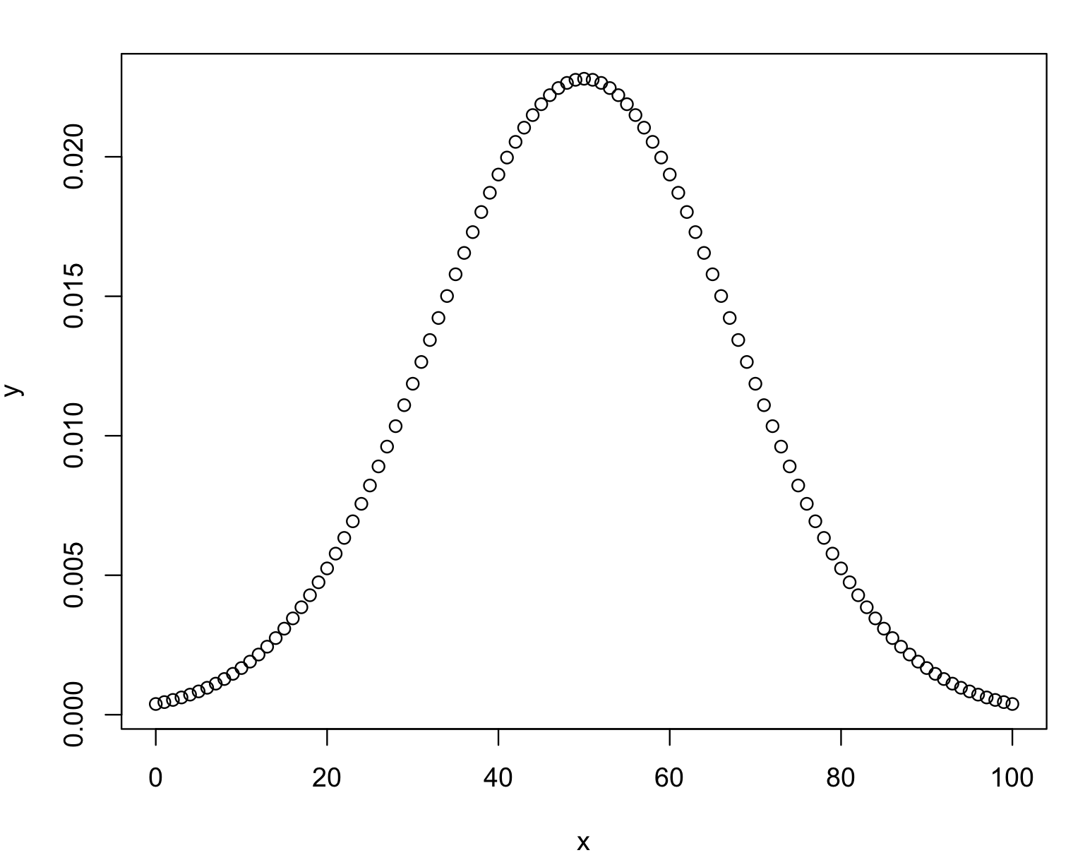
8) We can test for normal (Gaussian) distribution of our data using a normality test. We can use the Shapiro-Wilk’s test that determines if the null hypothesis (i.e., the sample has normal distribution) versus the alternative that it does not. If the test is significant, the distribution has a non-normal distribution. This test is sensitive to sample size, which means that large samples most often do not pass normality tests (i.e., show to be significant). Therefore, it’s important that you use visual inspection of your data distribution before you decide to transform your data.
The Shapiro-Wilk’s test is a build-in function and can be call as shapiro.test(). However, this test cannot be applied to large vectors (i.e., > 5000 entries).
# we can perfome in a variable of a data frame applying it as vector
shapiro.test(cars_data$hp)
#   Shapiro-Wilk normality test
#
#data:  cars_data$hp
#W = 0.93342, p-value = 0.04881
shapiro.test(cars_data$qsec)
#   Shapiro-Wilk normality test
#
#data:  cars_data$qsec
#W = 0.97325, p-value = 0.5935
Based on these results, we can conclude that the variable hp has not normal distribution, while qsec has normal one. If you want to apply the shapiro.test() to all you variables in your data frame use apply with 2 argument for columns.
apply(cars_data,2,shapiro.test)NOTICE the Shapiro-Wilk’s test is ONLY to test if your data is normally distributed, nothing else!!!.
9) In most cases, you might like to apply a transformation to your data before you apply a parametric statistical test. One of the most frequent transformations for continuous data is to normalize them, this means that change the distribution of the data to a quasinormal or normal one. Such transformations will make our data more amenable for parametric tests. However, the interpretation of the results has to be framed using the units of the transformed data (i.e., if log-transformed, you have to interpret in log-transformed unit).
To determine how if your data need to be normalized, it is a good idea to visualize its distribution. To exemplify this, we will describe this using the hp variable of the car_data.
hp_vector <- cars_data$hp
hp_vector
#[1] 110 110 93 110 175 105 245 62 95 123 123 180 180 180 205 215 230 66 52 65 97 150 150 245 175 66 91 113 264 175 335 109
# we test for normality
shapiro.test(hp_vector)
# Shapiro-Wilk normality test
#
#data: cars_data$hp
#W = 0.93342, p-value = 0.04881
boxplot(hp_vector, xlab = "hp", ylab = "values")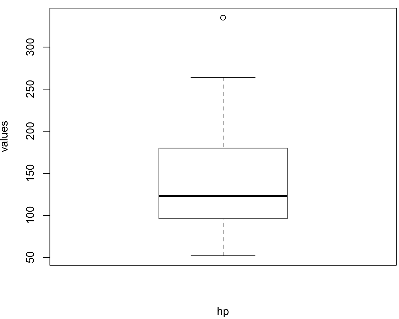 In this boxplot, we can see an outlier and it is skewed towards lower values of
 hp. Some of the most common transformations are to square root the data using the function sqrt() and to perform logarithms using log10() with base 10 or natural logarithms ‘log()’.
hp_vector_sqrt <- sqrt(hp_vector)
shapiro.test(hp_vector_sqrt)
#Shapiro-Wilk normality test
#
#data: hp_vector_sqrt
#W = 0.96456, p-value = 0.3642
hp_vector_log10 <- log10(hp_vector)
shapiro.test(hp_vector_log10)
# Shapiro-Wilk normality test
#
#data: hp_vector_log10
#W = 0.97026, p-value = 0.5065
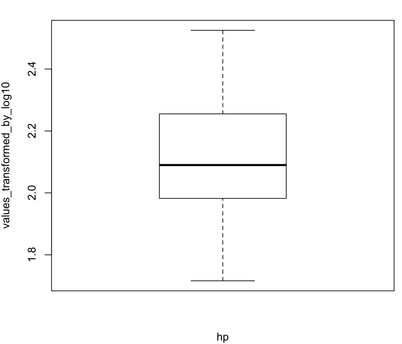
boxplot(hp_vector_log10, xlab = "hp", ylab = "values_transformed_by_log10")Here is the resulting boxplot afterlog10() transformation.
In some extreme cases, there are several R-packages that can help you to transform your data to have a normal distribution. One of these is bestNormalize and its function boxcox(). This provides a Box-Cox power transformation that can be useful for extremely skewed distributions. Likewise, this function returns, by default, transformed values that are also centered and scaled.
# if you need to install the R-package bestNormalize
install.packages("bestNormalize")
# load library
library(bestNormalize)
# perform Box-Cox power tranformation.
hp_vector_boxcox_list <- bestNormalize::boxcox(hp_vector)
hp_vector_boxcox_list
#Standardized Box Cox Transformation with 32 nonmissing obs.:
# Estimated statistics:
# - lambda = 0.0940865
# - mean (before standardization) = 6.21272
# - sd (before standardization) = 0.7515468
str(hp_vector_boxcox_list)
#List of 8
# $ x.t        : num [1:32] -0.401 -0.401 -0.745 -0.401 0.582 ...
#$ x          : num [1:32] 110 110 93 110 175 105 245 62 95 123 ...
#$ mean       : num 6.21
#$ sd         : num 0.752
#$ lambda     : num 0.0941
#$ n          : int 32
#$ norm_stat  : num 1.4
#$ standardize: logi TRUE
#- attr(*, "class")= chr [1:2] "boxcox" "list"
hp_vector_boxcox <- hp_vector_boxcox_list$x.t
hp_vector_boxcox
#(1] -0.4005863 -0.4005863 -0.7454816 -0.4005863  0.5821478 -0.4967035  1.3216259 -1.5563448 -0.7020701 -0.1680641 -0.1680641  0.6431660  0.6431660  0.6431660  0.9269679
#[16]  1.0317736  1.1809841 -1.4333227 -1.8985905 -1.4634315 -0.6594788  0.2511055  0.2511055  1.3216259  0.5821478 -1.4333227 -0.7897473 -0.3447992  1.4889763  0.5821478
#[31]  2.0305623 -0.4194885
boxplot(hp_vector_boxcox, xlab = "hp", ylab = "values_transformed_by_boxcox")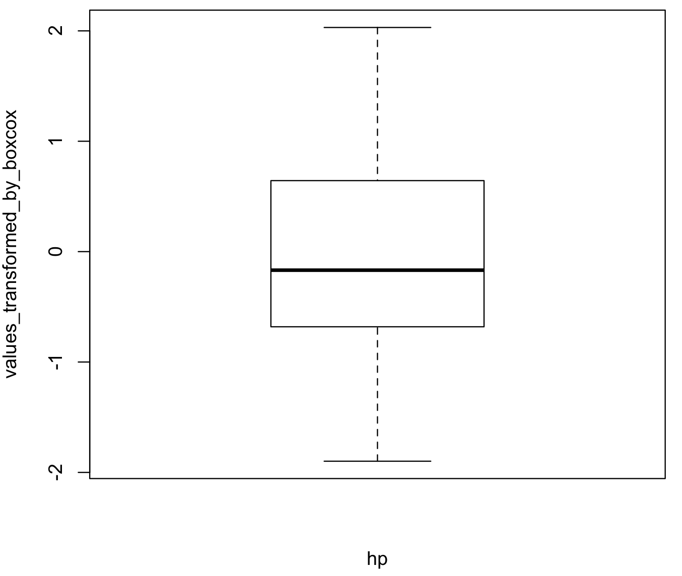
6.9 What test should I use?
The task of choosing the best statistical analyses given your dataset are one of the most important steps for any biological research. Your choice of methods depends on your understanding of your dataset and these include the following: (a) the number of dependent or outcome variables; (b) the number of your independent or predictor variables; (c) the characteristics of your dependent and independent variables, namely whether they are continuous (interval or ratio) variables (e.g., temperature, growth area, enzyme activity, dose amount, reaction rate, concentration, weight, length); (d) they are ordinal variables where order matters but differences between adjacent categories do not necessarily have the same meaning such as in treatment response (“low”, ”middle”, ”high”) or location (“understory”, “canopy”); (e) they are categorical variables if the categories that do not have a natural order or ranking such in colors (e.g., red, blue, green), populations (e.g., A, B, C, D); and (f) the type of distribution of the variables (it is normally distributed so parametric methods could be applied or not).
The table of statistical choices has been modified form here.
| Dependents (Number) | Dependents (Type) | Independents (Number) | Independents (Type) | Test | Section |
|---|---|---|---|---|---|
| 1 & one population | continuous (normal) | N/A | N/A | one-sample t-test | 6.11 |
| 1 & two populations | continuous (normal) | N/A | N/A | two-sample t-test | 6.12 |
| 1 & one population | continuous (non-normal); ordinal | N/A | N/A | one-sample median or Wilcoxon signed rank test | 6.13 |
| 1 & two populations | continuous (non-normal); ordinal | N/A | N/A | two-sample median or Wilcoxon signed rank test | 6.13 |
| 1 & one population | categorical (2 categories) | N/A | N/A | binomial test | 6.15 |
| 1 & one population | categorical (multiple categories) | N/A | N/A | Chi-square goodness-of-fit | 6.16 |
| 1 & two populations | categorical (multiple categories) compare agreements | N/A | N/A | Chi-square goodness-of-fit | 6.16 |
| 1 & two populations | categorical (multiple categories) | N/A | N/A | McNemar’s test | 6.17 |
| 1 & two populations | categorical (multiple categories) | N/A | N/A | Fisher’s exact test | 6.18 |
| 1 & one population | continuous (normal) | 1 | continuous (normal) | correlation | 6.19 |
| Comparing distributions | 6.20 | ||||
| Bootstraps | 6.21 | ||||
| 1 & one population | continuous (normal) | 1 | continuous (normal) | simple linear regression | 7.1 |
| 1 & one population | continuous (normal) | many | continuous (normal) | multiple linear regression | 7.3 |
| 1 & one population | ordinal | 1 | continuous or ordinal | simple logistic regression | 7.9 |
| 1 & one population | continuous | 1 | continuous or ordinal | non-parametric correlation | 7.11 |
| 1 & one population | continuous (normal) | 1 | categorical (2 or more categories) | one-way ANOVA | 7.13 |
| 1 & one population | continuous (non-normal); ordinal | 1 | categorical (2 or more categories) | one-way ANOVA | 7.14 |
| 1 & one population | continuous (normal) | 2 | categorical (2 or more categories) | two-way ANOVA | 7.15 |
| 1 & one population | continuous (non-normal) | 2 | categorical (2 or more categories) | Kruskal-Wallis Test | 7.17 |
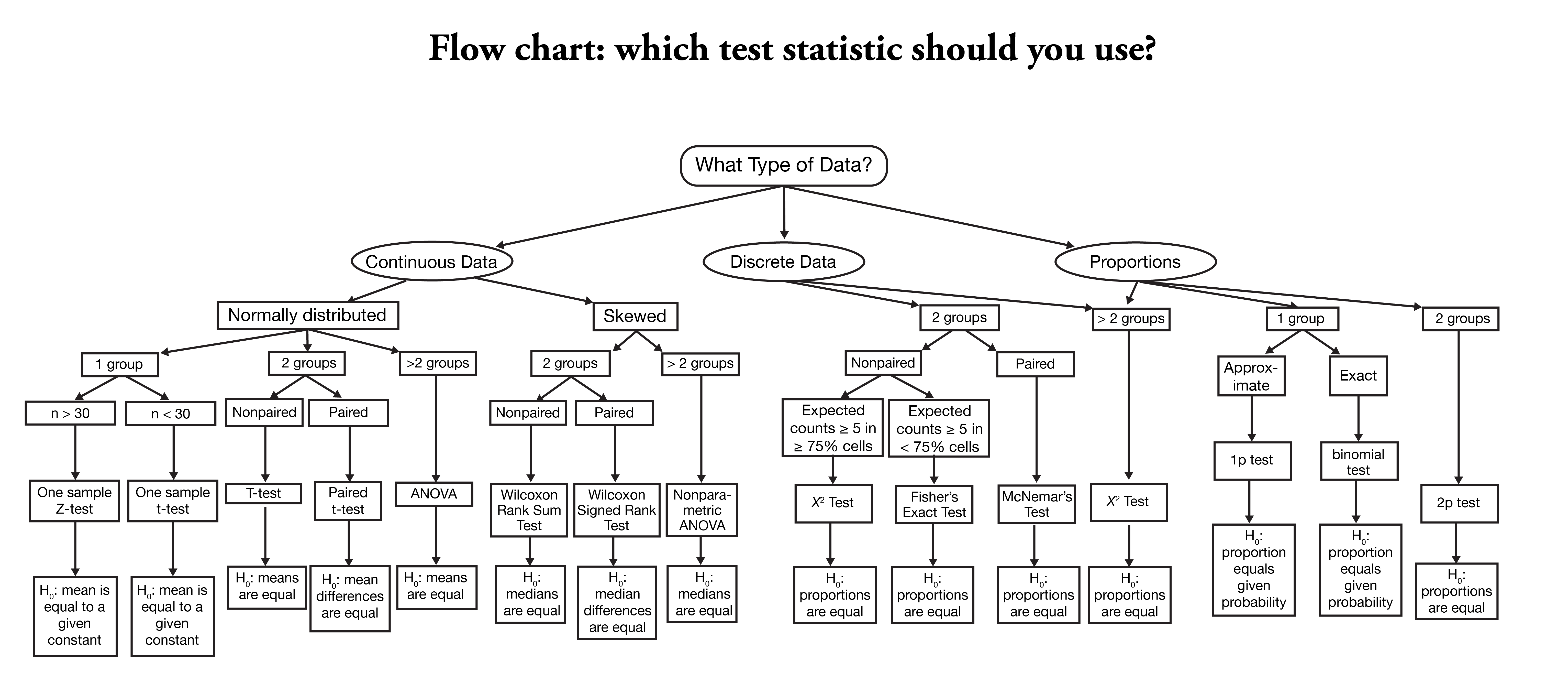
Here is another chart about selecting a statistial test for your project. The original source is in here.
6.10 Type of variables in dataset
You need to determine what type of variables do you have in your dataset. This is crucial if you want to use the correct test in the table above. It is very common that students fail to explore their data and plan to
force a test on their data without knowing (i.e., exploring!!!) if the variables in your dataset are continuous, discrete,
categorical, and binomial. We can easily check variable type by checking the data structure with str function.
## we can check the structure of car dataset by loading get mtcars dataset -- this a preloaded dataset in R
cars_data <- mtcars

## we add the 'car brand' as a character variable named 'brand'.
cars_data$brand <- rownames(cars_data)

## get the type of variable

str(cars_data)
#'data.frame':  32 obs. of  12 variables:
# $ mpg  : num  21 21 22.8 21.4 18.7 18.1 14.3 24.4 22.8 19.2 ...
# $ cyl  : num  6 6 4 6 8 6 8 4 4 6 ...
# $ disp : num  160 160 108 258 360 ...
# $ hp   : num  110 110 93 110 175 105 245 62 95 123 ...
# $ drat : num  3.9 3.9 3.85 3.08 3.15 2.76 3.21 3.69 3.92 3.92 ...
# $ wt   : num  2.62 2.88 2.32 3.21 3.44 ...
# $ qsec : num  16.5 17 18.6 19.4 17 ...
# $ vs   : num  0 0 1 1 0 1 0 1 1 1 ...
# $ am   : num  1 1 1 0 0 0 0 0 0 0 ...
# $ gear : num  4 4 4 3 3 3 3 4 4 4 ...
# $ carb : num  4 4 1 1 2 1 4 2 2 4 ...
# $ brand: chr  "Mazda RX4" "Mazda RX4 Wag" "Datsun 710" "Hornet 4 Drive" ...

## how many variables are numeric
sum(sapply(cars_data, is.numeric))
#[1] 11

## how many variables are character
sum(sapply(cars_data, is.character))
#[1] 1

## how many variables are factors
sum(sapply(cars_data, is.factor))
#[1] 0

## we can do a linear regreassion with mpg as dependent and disp, hp and wt as predictors
example_regression <- lm(mpg ~ disp + hp + wt, data = cars_data)
summary(example_regression)
# Call:
# lm(formula = mpg ~ disp + hp + wt, data = cars_data)
#
# Residuals:
#   Min     1Q Median     3Q    Max
# -3.891 -1.640 -0.172  1.061  5.861
#
# Coefficients:
#             Estimate Std. Error t value Pr(>|t|)
# (Intercept) 37.105505   2.110815  17.579  < 2e-16 ***
# disp        -0.000937   0.010350  -0.091  0.92851
# hp          -0.031157   0.011436  -2.724  0.01097 *
# wt          -3.800891   1.066191  -3.565  0.00133 **
# ---
# Signif. codes:  0 ‘***’ 0.001 ‘**’ 0.01 ‘*’ 0.05 ‘.’ 0.1 ‘ ’ 1
#
# Residual standard error: 2.639 on 28 degrees of freedom
# Multiple R-squared:  0.8268,  Adjusted R-squared:  0.8083
# F-statistic: 44.57 on 3 and 28 DF,  p-value: 8.65e-11

## we found taht hp and wt are good predictors of the mpg variable. For more detials on regressions see Session 7.
We can see that this dataset has 12 variables, 11 of those are continuous as num and only one named brand is a discrete variable indicated as chr.
We can now test another type of datasets from the R-package MASS.
## we can install MASS and load the dataset for this example
install.packages("MASS")
library(MASS)

## Let's explore the Aids2 dataset
Aids2_raw <- Aids2
str(Aids2_raw)
#'data.frame':  2843 obs. of  7 variables:
# $ state  : Factor w/ 4 levels "NSW","Other",..: 1 1 1 1 1 1 1 1 1 1 ...
# $ sex    : Factor w/ 2 levels "F","M": 2 2 2 2 2 2 2 2 2 2 ...
# $ diag   : int  10905 11029 9551 9577 10015 9971 10746 10042 10464 10439 ...
# $ death  : int  11081 11096 9983 9654 10290 10344 11135 11069 10956 10873 ...
# $ status : Factor w/ 2 levels "A","D": 2 2 2 2 2 2 2 2 2 2 ...
# $ T.categ: Factor w/ 8 levels "hs","hsid","id",..: 1 1 1 5 1 1 8 1 1 2 ...
# $ age    : int  35 53 42 44 39 36 36 31 26 27 ..

## how many variables are numeric
sapply(Aids2_raw, is.numeric)
# state     sex    diag   death  status T.categ     age
#  FALSE   FALSE    TRUE    TRUE   FALSE   FALSE    TRUE
sum(sapply(Aids2_raw, is.numeric))
#[1] 3
Aids2_raw_numeric <- Aids2_raw[,sapply(Aids2_raw, is.numeric)]
str(Aids2_raw_numeric)
#data.frame':   2843 obs. of  3 variables:
# $ diag : int  10905 11029 9551 9577 10015 9971 10746 10042 10464 10439 ...
# $ death: int  11081 11096 9983 9654 10290 10344 11135 11069 10956 10873 ...
# $ age  : int  35 53 42 44 39 36 36 31 26 27 ...
head(Aids2_raw_numeric)

## how many variables are character
sapply(Aids2_raw, is.character)
#  state     sex    diag   death  status T.categ     age
#  FALSE   FALSE   FALSE   FALSE   FALSE   FALSE   FALSE
sum(sapply(Aids2_raw, is.character))
#[1] 0
Aids2_raw_character <- Aids2_raw[,sapply(Aids2_raw, is.character)]
head(Aids2_raw_character)
# data frame with 0 columns and 6 rows

## how many variables are factors
sapply(Aids2_raw, is.factor)
# state     sex    diag   death  status T.categ     age
#   TRUE    TRUE   FALSE   FALSE    TRUE    TRUE   FALSE
sum(sapply(Aids2_raw, is.factor))
#[1] 4
Aids2_raw_factor <- Aids2_raw[,sapply(Aids2_raw, is.factor)]
str(Aids2_raw_factor)
#'data.frame':  2843 obs. of  4 variables:
# $ state  : Factor w/ 4 levels "NSW","Other",..: 1 1 1 1 1 1 1 1 1 1 ...
# $ sex    : Factor w/ 2 levels "F","M": 2 2 2 2 2 2 2 2 2 2 ...
# $ status : Factor w/ 2 levels "A","D": 2 2 2 2 2 2 2 2 2 2 ...
# $ T.categ: Factor w/ 8 levels "hs","hsid","id",..: 1 1 1 5 1 1 8 1 1 2 ...
head(Aids2_raw_factor)

## we can get the corresponding information for each with ?
?Aids2
We can see 7 variables, 3 are continuous as int (for integer) including two that are
not very useful as dates including diag and death. The variable age corresponds to age at diagnosis.
Two variables could be binary and also coded as factors with 2-levels including sex (i.e., male or female)
and status (i.e., alive or dead). Two are categorical such as state (i.e., four states in Australia) and
T.categ has 8 categories for reported transmission category.
We can do some exploration and even a t-test for the continuous variable
## we can get the summary of the age category
summary(Aids2_raw$age)
#  Min. 1st Qu.  Median    Mean 3rd Qu.    Max.
#   0.00   30.00   37.00   37.41   43.00   82.00

## we can test if 35 years is the mean of age of diagnosis of this population
t.test(Aids2_raw$age, mu = 35)
# One Sample t-test
#
# data:  Aids2_raw$age
# t = 12.764, df = 2842, p-value < 2.2e-16
# alternative hypothesis: true mean is not equal to 35
# 95 percent confidence interval:
# 37.03901 37.77914
# sample estimates:
# mean of x
# 37.40907
## we rejected the hypothesis that the age mean value of diagnosis is 35. See t-test for more details on this test.
We can continue our exploration and test if males and females are equally diagnosed with AIDS.
## we can get the summary of the sex category
summary(Aids2_raw$sex)
#   F    M
#  89 2754

## we need to convert it first to a numeric vector and then to a table
sex_as_numeric <- as.numeric(Aids2_raw$sex)
class(sex_as_numeric)
#[1] "numeric"
sex_as_table <- table(sex_as_numeric)
names(sex_as_table) <- c("female","male")
sex_as_table
#female   male
#    89   2754
## we can test if males and females are equally infected (50/50).
chisq.test(sex_as_table, p = c(1/2, 1/2))
#
#   Chi-squared test for given probabilities
#
# data:  sex_as_table
# X-squared = 2498.1, df = 1, p-value < 2.2e-16
## we rejected the hypothesis that the both males and females are affected in the same proportion (i.e., 1/2 and 1/2). See Chi-squared test for more details.
6.11 Comparing means: t-test
9) This analsys help us to test whether the difference between the response of two groups is statistically significant or not. We can perform one sample t-test on vectors using the function t.test(). For this test, you can test if its mean is statistically different from a given value specified by the mu argument equal such expected mean value.
## we will test the mean of sample SRR1039508 equal to mu = 546.5 for
cars_data <- mtcars
names(cars_data)[7]
#[1] "qsec"
t.test(cars_data$qsec, mu = 11)
#
#   One Sample t-test
#
#data:  cars_data$qsec
#t = 21.681, df = 31, p-value < 2.2e-16
#alternative hypothesis: true mean is not equal to 11
#95 percent confidence interval:
# 17.20449 18.49301
#sample estimates:
#mean of x
#17.84875

## we will test the mean of sample SRR1039508 equal to mu = 546.5 for

#load get 'airway_scaledcounts.csv' dataset
airway_data <- read.table("~/Desktop/Teach_R/class_pages_reference/bioinformatics_gitbook_1/my_working_directory/airway_scaledcounts.csv",
               header = TRUE, sep = ",", stringsAsFactors = FALSE)
names(airway_data)[2]
#[1] "SRR1039508"
t.test(airway_data[,2], mu = 546.5)
#
#   One Sample t-test
#
#data:  airway_data[, 2]
#t = -0.00053579, df = 38693, p-value = 0.9996
#alternative hypothesis: true mean is not equal to 546.5
#95 percent confidence interval:
# 501.7696 591.2060
#sample estimates:
#mean of x
# 546.4878
These result indicate that the mean of qsec from the cars_data is statically different form 11, while the mean for sample SRR1039508 from the airway_data is not different from the value 546.6 (this value was derived from the summary see 2)). One sample t-test does not assume that the population is normally distributed. However, it is better to have a normalized distribution in our data when we apply parametric test like this one.
The output of the function t.test() also provides 95% confidence interval of the mean value. In these examples, qsec has a mean 17.84875 with 95CI (17.20449, 18.49301) and the SRR1039508 sample mean is 546.4878 with 95CI (501.7696, 591.2060). Our interpretation is that the true value for the mean of the measurements of each of these variables is in the proposed range with a 95% confidence level.
Alternative analysis using the R-package lsr, which is specialized package for “Learning Statistics with R”.
## install package 'lsr'

install.packages("lsr")
library(lsr)

## we will use the same datasets

cars_data <- mtcars
names(cars_data)[7]
#[1] "qsec"

## one sample t-test
oneSampleTTest( x=cars_data$qsec, mu = 11)
#
#   One sample t-test
#
#Data variable:   cars_data$qsec
#
#Descriptive statistics:
#              qsec
#   mean     17.849
#   std dev.  1.787
#
#Hypotheses:
#   null:        population mean equals 11
#   alternative: population mean not equal to 11
#
#Test results:
#   t-statistic:  21.681
#   degrees of freedom:  31
#   p-value:  <.001
#
#Other information:
#   two-sided 95% confidence interval:  [17.204, 18.493]
#   estimated effect size (Cohen's d):  3.833
This output is very detailed including the same statistics as the previous t-test in R, but also includes more descriptive values such as mean, variance, confidence interval, and effect size. It also makes it explicit what is the null and alternative hypotheses; such that we consider that null mean is 11 while the alternative is different from 11 for ‘qsec’. The interpretation of the results is test is statistically significant (i.e., p-value <0.01). The interpretation of this result is that the actual mean ‘qsec’ of 17.849 for the group of 32 cars in our dataset have a much higher mean ‘qsec’ than the hypothesized mean value of 11 (t(31)=21.681, p-value < 0.001) with a 95% confidence interval of the mean value between 17.204 and 18.493. Notice the t(31) indicates that the t-statistic that has 31 degrees of freedom (i.e., 32 - 1 = 31).
6.12 Two sample t-test
10) For two samples, we can also perform t-tests with two vectors using the same function t.test(). In this case, you are testing if two samples each from different populations (e.g., control and experimental) have the same mean. If the test is significant, you can conclude that the difference might derive from a treatment (as long as you have controlled for other causal agents). These t-tests can be consider as paired (i.e., argument paired = TRUE) or unpaired (i.e., argument paired = FALSE). For paired, the t-test will compare the means of the same group under two separate conditions. In contrast, an unpaired t-test compares the means of two independent groups. In an unpaired t-test, the variance between groups is assumed to be equal.
We will use an unpaired t-test for Cars93 data from MASS to compare the Horsepower variable. Unparied is set by the argument paired = FALSE.
## we can install MASS and load the dataset for this example
install.packages("MASS")
library(MASS)
# We assign Cars93 dataset to an object
my_cars <- Cars93

# subset US and no_USA
US_cars <- subset(my_cars, Origin == "USA")
NonUS_cars <- subset(my_cars, Origin == "non-USA")
names_pairs <- c("US..vs..Non_US")

# get vectors for Horsepower
US_cars_Horsepower <- US_cars$Horsepower
NonUS_cars_Horsepower <- NonUS_cars$Horsepower

# mean value for Horsepower
mean(US_cars_Horsepower)
#[1] 147.5208
mean(NonUS_cars_Horsepower)
#[1] 139.8889

# do our unpaired t-test

out_put_ttest_paired <- t.test(US_cars_Horsepower, NonUS_cars_Horsepower, paired = FALSE)
cat(names_pairs); print(out_put_ttest_paired)
#US..vs..Non_US
#   Welch Two Sample t-test

#data:  US_cars_Horsepower and NonUS_cars_Horsepower
#t = 0.7021, df = 90.985, p-value = 0.4844
#alternative hypothesis: true difference in means is not equal to 0
#95 percent confidence interval:
# -13.96045  29.22433
#sample estimates:
#mean of x mean of y
# 147.5208  139.8889

## using the package 'lsr'two sample t-test
library(lsr)

# create a data frame for test

US_cars_Horsepower_df <- data.frame(hp = US_cars_Horsepower, maker = "US")
NonUS_cars_Horsepower_df <- data.frame(hp = NonUS_cars_Horsepower, maker = "No_US")
cars_hp_df <- rbind(US_cars_Horsepower_df,NonUS_cars_Horsepower_df)
cars_hp_df$maker <- factor(cars_hp_df$maker)
head(cars_hp_df)
#   hp maker
#1 110    US
#2 170    US
#3 180    US
#4 170    US
#5 200    US
#6 295    US

# two sample t-test
independentSamplesTTest( hp ~ maker, cars_hp_df, var.equal = FALSE)
#
#   Welch's independent samples t-test
#
#Outcome variable:   hp
#Grouping variable:  maker
#
#Descriptive statistics:
#              No_US      US
#   mean     139.889 147.521
#   std dev.  50.371  54.455
#
#Hypotheses:
#   null:        population means equal for both groups
#   alternative: different population means in each group
#
#Test results:
#   t-statistic:  -0.702
#   degrees of freedom:  90.985
#   p-value:  0.484
#
#Other information:
#   two-sided 95% confidence interval:  [-29.224, 13.96]
#   estimated effect size (Cohen's d):  0.146
The above results suggest that there is no difference between in the horsepower between these two types of cars based on their origin US versus Non-US.
Now, we will use a similar t-test this for airway_data dataset that has several transcriptome experiments and compare the mean expression and assumed that are the same population under two conditions using the argument paired = TRUE.
names_pairs <- names(airway_data)[2:3]
names_pairs <- paste0(names_pairs, collapse = "..vs..")
#[1] "SRR1039508..vs..SRR1039509"
out_put_ttest_paired <- t.test(airway_data[,2], airway_data[,3], paired = TRUE)
cat(names_pairs); print(out_put_ttest_paired)
#SRR1039508..vs..SRR1039509
#   Paired t-test
#
#data:  airway_data[, 2] and airway_data[, 3]
#t = 6.9876, df = 38693, p-value = 2.842e-12
#alternative hypothesis: true difference in means is not equal to 0
#95 percent confidence interval:
# 32.66123 58.12758
#sample estimates:
#mean of the differences
#               45.3944
The above results suggest that there is strong difference between these two samples of the same group.
Now, we will also consider the case of unpaired for comparison.
out_put_ttest_unpaired <- t.test(airway_data[,2], airway_data[,3], paired = FALSE)
cat(names_pairs); print(out_put_ttest_unpaired)
#SRR1039508..vs..SRR1039509
#   Welch Two Sample t-test
#
#data:  airway_data[, 2] and airway_data[, 3]
#t = 1.5108, df = 75614, p-value = 0.1309
#alternative hypothesis: true difference in means is not equal to 0
#95 percent confidence interval:
# -13.49803 104.28683
#sample estimates:
#mean of x mean of y
# 546.4878  501.0934
In this case, the result is the opposite and there is no evidence of a difference in the mean values if these samples were considered of different groups.
Note that a careful determination of what parametrization of the t-test is determined by your experimental group and other considerations. Likewise, a t-test is invalid for small samples from non-normal distributions, but it is valid for large samples from non-normal distributions (like our example above with >30,000 entries). These considerations are beyond this bioinformatics workshop and are the topic of a biostatistics course.
6.13 Beyond t-test: Wilcoxon signed rank test
11) Alternatives to the parametric t-test exist, one of the most common is the one/two-sample median test or the Wilcoxon signed rank test. This test is used to compare two unpaired and paired samples or repeated measurements on a single sample to assess whether their population mean ranks differ.
The Wilcoxon signed rank test is implemented with the function wilcox.test() in a similar fashion as is in a t.test().
# test for mean of sample

wilcox.test(cars_data$qsec, mu = 11)
# Wilcoxon signed rank test with continuity correction
#
# data:  cars_data$qsec
# V = 528, p-value = 8.334e-07
# alternative hypothesis: true location is not equal to 11

wilcox.test(airway_data[,2], mu = 546.5)
#
#   Wilcoxon signed rank test with continuity correction
#
#data:  airway_data[, 2]
#V = 145919557, p-value < 2.2e-16
#alternative hypothesis: true location is not equal to 546.5

# test for two samples of different group
wilcox.test(airway_data[,2], airway_data[,3], paired = FALSE)
#
#   Wilcoxon rank sum test with continuity correction
#
#data:  airway_data[, 2] and airway_data[, 3]
#W = 753579582, p-value = 0.08979
#alternative hypothesis: true location shift is not equal to 0

# test for two samples of same group, paired-test
wilcox.test(airway_data[,2], airway_data[,3], paired = TRUE)
#
#   Wilcoxon signed rank test with continuity correction
#
#data:  airway_data[, 2] and airway_data[, 3]
#V = 147963112, p-value < 2.2e-16
#alternative hypothesis: true location shift is not equal to 0
6.14 Tabulation and Cross-Tabulation
Some data analyses require that the information be in the form of frequency tables or cross-tabulation of one variable against another.
We can explore some functions to help us with tabulation: table() and xtabs(). We can start with a vector of repeated values that can be included in a table.test
## we create two vectors of some values

vector_colors <- c("red","red","black","blue","green","green","green","green","blue","blue","blue","blue","blue")
str(vector_colors)
#chr [1:13] "red" "red" "black" "blue" "green" "green" "green" "green" "blue" "blue" "blue" "blue" "blue"

vector_numbers <- c(1,1,1,2,2,2,2,3,3,3,3,4,4,4,4,4,4,6,6,6,6,6,6,6,6)
str(vector_numbers)
# num [1:25] 1 1 1 2 2 2 2 3 3 3 ...
you can also create such vectors of repeated elements if you know how many times each is repeated using the function rep() to replicate elements of vectors.
## we recreate two vectors from above


vector_color_names <- c("black","blue","green","red")
number_color_is_repeated <- c(1,6,4,2)
vector_colors <- rep(vector_color_names, number_color_is_repeated)
str(vector_colors)
#chr [1:13] "black" "blue" "blue" "blue" "blue" "blue" "blue" "green" "green" "green" "green" "red" "red"


vector_value_names <- c(1,2,3,4,6)
number_value_is_repeated <- c(3,4,4,6,8)
vector_numbers <- rep(vector_value_names, number_value_is_repeated)
str(vector_numbers)
# num [1:25] 1 1 1 2 2 2 2 3 3 3 ...
We now can create table object using the function table(). These tables contain a frequency count of the number of times that a unique elements on each vector is repeated.
## we create table objects using the two previous vectors

table_numbers <- table(vector_numbers)
table_numbers
# vector_numbers
#1 2 3 4 6
#3 4 4 6 8

table_colors <- table(vector_colors)
table_colors
# vector_colors
# black  blue green   red
#    1     6     4     2
These table objects contain three lines. The first line tell us that we are looking at a tabulation of the vector named: vector_numbers and vector_colors.
On the second line it lists all the different elements such as unique numbers (i.e., 1,2,3,4,6) or colors (i.e., black, blue, green, red) that exist in each vector, and on the third line it tells
you how many times that each unique element appears in the data.
We can create a cross-tabulation, if we have two or more vectors that have the same number of elements and tells us when the two elements (one for the first vector and one for the second vector) cooccur.
vaccinated_vector        <- c("YES","NO","YES","YES","YES","YES","YES","NO","NO","YES","NO","YES","NO")
table(vaccinated_vector)
#vaccinated_vector
# NO YES
#  5   8

healthy_0_sick_1_vector  <- c( 0,    1,   0,     1,    1,    0,    0,   1,    0,  0,    1,  0,  1)
table(healthy_0_sick_1_vector)
#healthy_0_sick_1_vector
#0 1
#7 6

outcome_crosstab <- table(vaccinated_vector,healthy_0_sick_1_vector)
outcome_crosstab
#                 healthy_0_sick_1_vector
# vaccinated_vector 0 1
#               NO  1 4
#               YES 6 2
You can create tables from data frames. We will create a data.frame() from the example above.
vac_health_df <- data.frame(vaccinated_vector, healthy_0_sick_1_vector)
vac_health_df
#   vaccinated_vector healthy_0_sick_1_vector
#1                YES                       0
#2                 NO                       1
#3                YES                       0
#4                YES                       1
#5                YES                       1
#6                YES                       0
#7                YES                       0
#8                 NO                       1
#9                 NO                       0
#10               YES                       0
#11                NO                       1
#12               YES                       0
#13                NO                       1
We will add another variable to our data frame such as sex, remember that it has to have the same number of row as the data frame (i.e., 13).
sex <- c("m","f","m","f","f","f","f","f","f","m","m","m","m")
vac_health_df$sex <- sex
vac_health_df
#   vaccinated_vector healthy_0_sick_1_vector sex
#1                YES                       0   m
#2                 NO                       1   f
#3                YES                       0   m
#4                YES                       1   f
#5                YES                       1   f
#6                YES                       0   f
#7                YES                       0   f
#8                 NO                       1   f
#9                 NO                       0   f
#10               YES                       0   m
#11                NO                       1   m
#12               YES                       0   m
#13                NO                       1   m
Now you can select particular set of variables from the data frame to tabulate using the function xtabs(). In this function, you input a one sided formula in order to list all the variables you want to cross-tabulate, and the name of the data frame that stores the data.
## one variable

xtabs( formula = ~ vaccinated_vector, data = vac_health_df)
#vaccinated_vector
#NO YES
#  5   8
xtabs( formula = ~ healthy_0_sick_1_vector, data = vac_health_df)
#healthy_0_sick_1_vector
#0 1
#7 6
xtabs( formula = ~ sex, data = vac_health_df)
#sex
#f m
#7 6

## two variables cross-tabulation

xtabs( formula = ~ vaccinated_vector + healthy_0_sick_1_vector, data = vac_health_df)
#                 healthy_0_sick_1_vector
#vaccinated_vector 0 1
#              NO  1 4
#              YES 6 2

xtabs( formula = ~ vaccinated_vector + sex, data = vac_health_df)

#                 sex
#vaccinated_vector f m
#              NO  3 2
#              YES 4 4

## three variables cross-tabulation

xtabs( formula = ~ vaccinated_vector + healthy_0_sick_1_vector + sex, data = vac_health_df)

#, , sex = f
#
#                 healthy_0_sick_1_vector
#vaccinated_vector 0 1
#              NO  1 2
#              YES 2 2
#
#, , sex = m
#
#                 healthy_0_sick_1_vector
#vaccinated_vector 0 1
#              NO  0 2
#              YES 4 0
6.15 Beyond t-test: Binomial test
12) The binomial test will determine the significance of deviations from expected distribution of observations into two groups of categorical variable. One common use of this test is when an experiment has two possible outcomes (i.e. success/failure) and you have an expectation (i.e., probability) success. For example, if you flip fair coin you have expectation of 50/50 chance of heads of tail every flip. You can apply a binomial test to a population with two categories using the function prop.test().
For example, we can test if the number of females in a population is p = 0.51 (i.e., the chance of being female is 51%). We will use function rbinom() to create such population of 1000 individuals.
## we create a binomial variable assigned to males of females.
## we assume that if female is 1 and 0 if male

one_population <- rbinom(n = 1000, size = 1, prob= 0.51)
str(one_population)
#int [1:1000] 0 0 0 0 1 0 1 0 0 1 ...

## you can tabulate the data in your one_population to visualize that the data follows
## roughly the predicted proportion of 0-state (0.49 or 49%) and 1-state (0.51 or 51%)
table(one_population)
#one_population
#  0   1
#487 513

prop.table(table(one_population))

#one_population
#    0     1
#0.492 0.508

## we can perform the bionomial test for an expected value of propotion of 1 to be p = 0.51

prop.test(sum(one_population), length(one_population), p = 0.51)
#
#   1-sample proportions test with continuity correction
#
#data:  sum(one_population) out of length(one_population), null probability 0.51
#X-squared = 0.04902, df = 1, p-value = 0.8248
#alternative hypothesis: true p is not equal to 0.51
#95 percent confidence interval:
# 0.4745504 0.5374029
#sample estimates:
#    p
#0.506
In the case above, we found a non-significant result p-value = 0.8248 and this population is likely to have 51% chance of females.
However, we can create a biased population towards males with probability equal to 0.4 (i.e., males are 0 and females ar 1). In other words, females (represened by 1) will appear only 40% of time on the population the rest will be males (represented by 0).
## we create a binomial variable assigned to males of females.
## we assume that if female is 1 and 0 if male

other_population <- rbinom(n = 1000, size = 1, prob= 0.40)
str(other_population)
#int [1:1000] 0 0 0 0 1 1 0 1 0 0 ...

## you can tabulate the data in your one_population to visualize that the data follows
## roughly the predicted proportion of 0-state (0.60 or 60%) and 1-state (0.40 or 40%)
table(other_population)
#other_population
#  0   1
#603 397

## we can perform the binomial test

prop.test(sum(other_population), length(other_population), p = 0.51)
#
#   1-sample proportions test with continuity correction
#
#data:  sum(other_population) out of length(other_population), null probability 0.51
#X-squared = 45.387, df = 1, p-value = 1.617e-11
#alternative hypothesis: true p is not equal to 0.51
#95 percent confidence interval:
# 0.3725342 0.4342204
#sample estimates:
#    p
#0.403
In the case above, we found a significant result p-value = 1.617e-11 and this population unlikely has 51% chance of females.
6.16 Beyond t-test: Chi-square goodness of fit
13) The Chi-square goodness of fit test will determine the significance of deviations from expected probabilities of multiple categories in a population. For example, you might want to compare the observed distribution of categories of a population to an expected distribution of such categories.
We will perform this test using a table object with multiple categories with the function chisq.test() and an argument of probabilities for each category provided byp.
For example, we can test if the proportion of nitrogen fixing bacteria in a population collected of dataset rhizobium from R package ade4.
## load rhizobium dataset from ade4 R package
library(ade4)
data(rhizobium)
?rhizobium
rhizobium_pop <- as.character(rhizobium$pop)
str(rhizobium_pop)
#chr [1:215] "FTmdc" "FTmdc" "FTmdc" "FTmdc" "FTmdc" "FTmdc" "FTmdc" "FTmdc" "FTmdc" "FTmdc" "FTmdc" "FTmdc" "FTmdc" ...

## get a idea of the unique character elements in the rhizobium_pop object
unique(rhizobium_pop)
#[1] "FTmdc"  "FTmlt"  "TETmdc" "THLmlt" "TELmlt" "TETmlt" "THTmlt"

#we can see 7 unique text elements

## create a table object
rhizobium_pop_table <- table(rhizobium_pop)
rhizobium_pop_table
#rhizobium_pop
# FTmdc  FTmlt TELmlt TETmdc TETmlt THLmlt THTmlt
#    46     43     20     20     24     20     42

## we have 7 categories. We will assume that they should be in equal proportion (i.e., 1/7 each).
rhizobium_test <- chisq.test(rhizobium_pop_table, p = c(1/7, 1/7, 1/7, 1/7, 1/7, 1/7, 1/7))
rhizobium_test
#
#   Chi-squared test for given probabilities
#
#data:  rhizobium_pop_table
#X-squared = 29.349, df = 6, p-value = 5.225e-05

# observed counts for each rhizobium population
rhizobium_test$observed
# FTmdc  FTmlt TELmlt TETmdc TETmlt THLmlt THTmlt
#    46     43     20     20     24     20     42


# expected counts for each rhizobium population under the null hypothesis of 1/7 for each one
rhizobium_test$expected
#   FTmdc    FTmlt   TELmlt   TETmdc   TETmlt   THLmlt   THTmlt
#30.71429 30.71429 30.71429 30.71429 30.71429 30.71429 30.71429
14) You can also cross tabulate results of two measurements of population that result in two or more categories for each and determine if they are related using a Chi-square goodness of fit test. The goal is to create a contingency table where your compare the outcomes for two different measurements of the same population and determine if they tend to be in agreement or not.
## we can have a population and determine a categorical variable that result in two category (0, 1) like for example: healthy and sick
sample_population <- rbinom(n = 100, size = 1, prob= 0.40)
population_states <- ifelse(sample_population  == 1, "sick", "healthy")
names(sample_population) <- population_states
head(sample_population)
#  healthy   sick healthy healthy healthy healthy
#      0       1       0       0       0       0

## we can have the same population and determine a different categorical variable that result in two categories (0, 1) like for example: with_virus and no_infected
sample_virus <- rbinom(n = 100, size = 1, prob= 0.40)
virus_names <- ifelse(sample_virus  == 1, "with_virus", "no_infected")
names(sample_virus) <- virus_names
head(sample_virus)
#    no_infected no_infected no_infected no_infected  with_virus no_infected
#          0           0           0           0           1           0
We cross-tabulate these results and it is important to understand this table. The outcomes for sample_population and sample_virus are 0 1 as indicated in the first row and column. The agreements are when the outcomes of both experiments are the same as each experiment was executed 0-0 and 1-1. All others are disagreements (e.g., 0-1, 1-0).
cross_tab <- table(sample_population, sample_virus)
cross_tab
#                 sample_virus
#sample_population  0  1
#                0 33 20
#                1 23 24
We can now estimate if such agreements and disagreements are different using Chi-squared Test for Count Data with the function chisq.test().
madeup_virus_test <- chisq.test(cross_tab)
madeup_virus_test
#
#   Pearson's Chi-squared test with Yates' continuity correction
#
# data:  cross_tab
# X-squared = 1.2956, df = 1, p-value = 0.255

# observed counts for sample_virus vs sample_population
madeup_virus_test$observed
#                 sample_virus
#sample_population  0  1
#                0 33 20
#                1 23 24

# Consider that we assume that each combination will have an equal probability to occur such as 0.25 for 4 combinations

rep(1/length(cross_tab), length(cross_tab))
#[1] 0.25 0.25 0.25 0.25

# expected counts for sample_virus vs sample_population under this null hypothesis
madeup_virus_test$expected

#                 sample_virus
#sample_population     0     1
#                0 29.68 23.32
#                1 26.32 20.68
In this case, we found that they were non-significant different. In this case, if the sick people might not have this made-up virus.
Here is another example, in this case we will make people that are sick more likely to have a virus (i.e., more healthy people will not have the virus).
#$ we construct a data frame
sample_virus_2 <- data.frame (population_1_if_sick = c(0,0,0,1,1,1,1,1,0,1,1),
                               virus_1_if_detected = c(0,0,0,1,1,1,1,0,0,1,1), stringsAsFactors = FALSE)
sample_virus_2
#   population_1_if_sick virus_1_if_detected
#1                     0                   0
#2                     0                   0
#3                     0                   0
#4                     1                   1
#5                     1                   1
#6                     1                   1
#7                     1                   1
#8                     1                   0
#9                     0                   0
#10                    1                   1
#11                    1                   1

## we save to numeric vectors
population_1_if_sick <- sample_virus_2$population_1_if_sick
virus_1_if_detected <- sample_virus_2$virus_1_if_detected

## we do a crosstabulation
cross_tab2 <- table(population_1_if_sick, virus_1_if_detected)
cross_tab2
#                    virus_1_if_detected
#population_1_if_sick 0 1
#                   0 4 0
#                   1 1 6

## we perform the chisq.test
virus_pop_results <- chisq.test(cross_tab2)

#Warning message:
#In chisq.test(cross_tab2) : Chi-squared approximation may be incorrect

virus_pop_results
#   Pearson's Chi-squared test with Yates' continuity correction
#
# data:  cross_tab2
# X-squared = 4.4818, df = 1, p-value = 0.03426
#
# Warning message:
# In chisq.test(cross_tab2) : Chi-squared approximation may be incorrect

virus_pop_results$observed
#                    virus_1_if_detected
#population_1_if_sick 0 1
#                   0 4 0
#                   1 1 6
virus_pop_results$expected
#                    virus_1_if_detected
#population_1_if_sick        0        1
#                   0 1.818182 2.181818
#                   1 3.181818 3.818182
We found that people sick most likely have the virus and this is significant. However, we notice a Warning and this is because of expected values that are more than 5 are usually required to fulfill chisq.test assumptions. Consider using Fisher’s exact test.
6.17 Beyond t-test: McNemar’s test
15) This is a similar test to the Chi-square goodness of fit and it is used with paired nominal data in 2 × 2 contingency tables derived from dichotomous trait (i.e., YES or NO; Present or Absent), with matched pairs of subjects, to determine whether the row and column marginal frequencies are equal (see here).
## we can use the same cross tabulation example
cross_tab <- table(sample_population, sample_virus)
cross_tab
#                 sample_virus
#sample_population  0  1
#                0 33 20
#                1 23 24

## we apply the McNemar's test

madeup_virus_test_mcnemar <- mcnemar.test(cross_tab)
madeup_virus_test_mcnemar
#
#       McNemar's Chi-squared test with continuity correction
#
#data:  cross_tab
#McNemar's chi-squared = 0.093023, df = 1, p-value = 0.7604
In this case, we found that the same result as the Chi-squared test and McNemar-s test was also non-significant. In this case, if the sick people might not have this made-up virus.
6.18 Beyond t-test: Fisher’s exact test
16) This is a similar test to the Chi-square goodness of fit and can be used with populations with small samples. The Fisher’s exact test will examine the significance of the association (contingency) between the two kinds of classification. The null hypothesis is that both classifications are dependent. We can use the same dataset as above with the function fisher.test().
## for the virus_pop_results
madeup_virus_test_fisher <- fisher.test(cross_tab)
madeup_virus_test_fisher
#
#       Fisher's Exact Test for Count Data
#
#data:  cross_tab
#p-value = 0.227
#alternative hypothesis: true odds ratio is not equal to 1
#95 percent confidence interval:
# 0.7205596 4.1251469
#sample estimates:
#odds ratio
#  1.712314
These results are non significant. This result is similar to the chisq.test results.
## for the virus_pop_results
virus_pop_results_fisher <- fisher.test(cross_tab2)
virus_pop_results_fisher
#   Fisher's Exact Test for Count Data
#
#data:  cross_tab2
#p-value = 0.01515
#alternative hypothesis: true odds ratio is not equal to 1
#95 percent confidence interval:
# 1.269441      Inf
#sample estimates:
#odds ratio
#       Inf
In this case, we find that people sick most likely have the virus and this is significant. This result is similar to the chisq.test results.
6.19 Correlations
17) We can determine correlation between two variables using cor() and test for its significance using cor.test(). Correlation is the dependence or association between variables, and it usually refers to the degree to which a pair of variables are linearly related. For practical uses, correlations can provide a predictive relationship that can derived from one variable on the other. However, the evidence of correlation does not mean a causal relationship (i.e., A does not necessarily cause B and viceversa). Likewise, it is important to determine if such correlations are significant and these can be performed for normal or non-normal distributions (in this case use the use argument method = "spearman").
We will determine a correlation and test for its significance between two samples of the airway_data.
cars_data <- mtcars
head(cars_data)
#                   mpg cyl disp  hp drat    wt  qsec vs am gear carb
#Mazda RX4         21.0   6  160 110 3.90 2.620 16.46  0  1    4    4
#Mazda RX4 Wag     21.0   6  160 110 3.90 2.875 17.02  0  1    4    4
#Datsun 710        22.8   4  108  93 3.85 2.320 18.61  1  1    4    1
#Hornet 4 Drive    21.4   6  258 110 3.08 3.215 19.44  1  0    3    1
#Hornet Sportabout 18.7   8  360 175 3.15 3.440 17.02  0  0    3    2
#Valiant           18.1   6  225 105 2.76 3.460 20.22  1  0    3    1

# test correlation between weight and mpg
cor(cars_data$wt, cars_data$mpg)
#[1] -0.8676594
cor.test(cars_data$wt, cars_data$mpg, method = "pearson")
#
#   Pearson's product-moment correlation
#
#data:  cars_data$wt and cars_data$mpg
#t = -9.559, df = 30, p-value = 1.294e-10
#alternative hypothesis: true correlation is not equal to 0
#95 percent confidence interval:
# -0.9338264 -0.7440872
#sample estimates:
#       cor
#-0.8676594


cor(airway_data[,2], airway_data[,3])
#[1] 0.9646265
# we will assume that these are not normal
cor.test(airway_data[,2], airway_data[,3], method = "spearman")
#
#   Spearman's rank correlation rho
#
#data:  airway_data[, 2] and airway_data[, 3]
#S = 4.8345e+11, p-value < 2.2e-16
#alternative hypothesis: true rho is not equal to 0
#sample estimates:
#      rho
#0.9499302
6.20 The MAGIC criteria
This is a set of considerations for the results of many statistical analyses and they indicate their relevance for ‘real life’ inferences. It was proposed by Robert Abelson from his book Statistics as Principled Argument. These criteria suggest that the goal of statistical analysis should be to make compelling to be meaningful inferences of real-life considerations. It goes beyond the significance of the p-value, and helps to determine if we should care if the study has a practical value.
The MAGIC criteria is a backronym for:
Magnitude – How big is the effect? Large effects are more compelling than small ones.
Articulation – How specific is it? Precise statements are more compelling than imprecise ones.
Generality – How generally does it apply? More general effects are more compelling than less general ones. Claims that would interest a more general audience are more compelling.
Interestingness – Interesting effects are those that “have the potential, through empirical analysis, to change what people believe about an important issue”. More interesting effects are more compelling than less interesting ones. In addition, more surprising effects are more compelling than ones that merely confirm what is already known.
Credibility – Credible claims are more compelling than incredible ones. The researcher must show that the claims made are credible. Results that contradict previously established ones are less credible.
6.21 Effect size
This collection of statistics measures the magnitude of a difference or strength of the relationship between variables. It helps determine the practical significance of the study results as referred in the MAGIC criteria. In other words, it allows you to see beyond just statistical significance of the p-values, determine its practical value, and it is not affected by sample size.
For t-tests, you can use Cohen’s d that measures the difference between two means in terms of standard deviation. For correlations, you can use the Pearson-correlation (also known as r) measurement of the strength of correlation between two variables, similarly you can use the coefficient of determination (r2 or R2 or “r-squared”), calculated as the square of the Pearson correlation r. For ANOVA, you can use eta-squared to measure the proportion of variance explained by an independent variable.
| Effect size | Cohen’s d | Pearson’s r | R-squared |
|---|---|---|---|
| Small | 0.01 - 0.20 | 0.05 - 0.10 | 0.01 - 0.09 |
| Medium | 0.20 - 0.50 | 0.10 - 0.30 | 0.09 - 0.25 |
| Large | 0.50 - 0.80 | 0.30 - 0.40 | >0.25 |
| Very Large | >0.80 | >0.40 | >0.25 |
Effect sizes can help to determine if the sample size in your study is good enough or needs to be increased. Likewise, when combining or comparing multiple independent studies (e.g., meta-analysis) the effect size of each can be used to weigh their contribution, so that large sample-size studies are given more weight (i.e., they are more important) than small sample-size studies. You must try to report effect sizes of your tests (if possible) such to facilitate the interpretation of the importance of your research beyond mere statistical significance.
For t-tests, you can use the function cohensD for the R-package lsr
library(lsr)

## we will use the same dataset

cars_data <- mtcars

## one sample t-test with mu = 11

cohensD( x=cars_data$qsec, mu = 11)
#[1] 3.832662

## for two sample t-test comparing the mean

library(MASS)

my_cars <- Cars93
US_cars <- subset(my_cars, Origin == "USA")
NonUS_cars <- subset(my_cars, Origin == "non-USA")
US_cars_Horsepower <- US_cars$Horsepower
NonUS_cars_Horsepower <- NonUS_cars$Horsepower
US_cars_Horsepower_df <- data.frame(hp = US_cars_Horsepower, maker = "US")
NonUS_cars_Horsepower_df <- data.frame(hp = NonUS_cars_Horsepower, maker = "No_US")
cars_hp_df <- rbind(US_cars_Horsepower_df,NonUS_cars_Horsepower_df)
cars_hp_df$maker <- factor(cars_hp_df$maker)


cohensD( formula = hp ~ maker,  # horsepower ~ US versus Non-US cars
          data = cars_hp_df,    # data frame
          method = "unequal"     # which version to calculate?
        )
# [1] 0.1455011
In the first case (one sample t-test) the effect size was very large, while the other was small.
6.22 Comparing distributions
18) We can also determine if two variables come from the same distribution using Kolmogorov-Smirnov test ks.test(). The data does not require to be normal.
We will determine if two samples of the airway_data have the same distribution.
ks.test(airway_data[,2], airway_data[,3])
#
#   Two-sample Kolmogorov-Smirnov test
#
#data:  airway_data[, 2] and airway_data[, 3]
#D = 0.013413, p-value = 0.001896
#alternative hypothesis: two-sided
#
#Warning message:
#In ks.test(airway_data[, 2], airway_data[, 3]) :
#  p-value will be approximate in the presence of ties
We can conclude that these two samples do not have the same distribution (i.e., p-value = 0.001896).
19) We can compare two groups that have some individuals in such groups being exposed treatment versus control using
from the R-package pROC using the functions roc() and roc.test().
This test will compare the AUC (area under the curve) of two ROC (receiver operating characteristic) curves.
These are graphical plots useful in the diagnostic of a binary classifier (e.g., “control-0” or “exposed-1”) as its discrimination threshold is varied (i.e., what is the cutoff to consider a measurement as “exposed-1”).
We will illustrate this test using two airway_data by assigning “control” and “exposed” to sample of rows.
# you need to instal the package "pROC"
install.packages("pROC")
library(pROC)
We can prepare two samples of airway_data and assign some of elements of each as “control” and “exposed”.
## set two samples
sample_SRR1039508 <- airway_data$SRR1039508
sample_SRR1039509 <- airway_data$SRR1039509

## get summaries of each
summary_SRR1039508 <- summary(sample_SRR1039508)
summary_SRR1039508
#    Min.  1st Qu.   Median     Mean  3rd Qu.     Max.
#     0.0      0.0      1.0    546.5    203.0 287372.0
summary_SRR1039509 <- summary(sample_SRR1039509)
summary_SRR1039509
#    Min.  1st Qu.   Median     Mean  3rd Qu.     Max.
#     0.0      0.0      1.0    501.1    172.0 244921.0

## assign  "control" if less than 3rd quartile of each
SRR1039508_binary <- ifelse(sample_SRR1039508 > summary_SRR1039508[5], "exposed", "control")
## assign  "control" if more than 3rd quartile of each -- a reverse from last sample
SRR1039509_binary <- ifelse(sample_SRR1039509 > summary_SRR1039509[5], "control", "exposed")

## create a roc object for each sample
roc_SRR1039508 <- roc(SRR1039508_binary, sample_SRR1039508, direction = "<")
#Setting levels: control = control, case = exposed
roc_SRR1039509 <- roc(SRR1039509_binary, sample_SRR1039509, direction = "<")
#Setting levels: control = control, case = exposed

## perform the roc.test and increase boot.n for a more precise p-value:
roc.test(roc_SRR1039508, roc_SRR1039509, method="bootstrap", boot.n=1000)
#    |=========================================================================================================================================================================| 100%
#
#   Bootstrap test for two ROC curves
#
#data:  roc_SRR1039508 and roc_SRR1039509
#D = Inf, boot.n = 1000, boot.stratified = 1, p-value < 2.2e-16
#alternative hypothesis: true difference in AUC is not equal to 0
#sample estimates:
#AUC of roc1 AUC of roc2
#          1           0
We can conclude that for SRR1039508 and SRR1039509 are different in their distribution in reference to outcomes for “control” versus “exposed”.
6.23 Bootstraps
This is a non-parametric method of repeated resampling from collection of data with replacement. With enough sampling repetitions (usually in thousands), we can estimate the distribution of a parameter(s) of a population where an original data collection can be used a source for resampling. The rational is that with enough repeat sampling from this population of data, we likely obtain a distribution of values for a parameter (e.g., means, correlations, etc.) that we want to estimate from the population being studied. Repeated sampling allows to account for the uncertainty that resulted from a single or few samples. We calculate from this collection of samples a statistic of interest (e.g., mean) and with enough repetitions the shape of the distribution of the estimates of the statistic would be “bell shaped” (i.e., have Gaussian distribution), which makes possible to construct a confidence interval of our statistic.
Bootstrap can be done in R and it requires to have a source collection (usually large) of data from our population of interest that will serve to draw the bootstrap samples. We will define how many samples with replacement will be drawn (e.g., >1000), with a given sample size (i.e., how many elements are drawn during each sample usually). From each sample, we will estimate a parameter of interest (e.g., a mean) and collect those to calculate of distribution where its mean (expected value for the statistic) and standard deviation (a measure of the uncertainty about that value of the statistic) can be used to estimate a confidence interval of such statistic.
We need to install the R-package boot.
install.packages('boot')
library(boot)
We will use the mtcars to illustrate the estimate of mean and correlation between some of the variables.
#load get mtcars dataset -- this a preloaded dataset in R
cars_data <- mtcars
cars_data
#                     mpg cyl  disp  hp drat    wt  qsec vs am gear carb
#Mazda RX4           21.0   6 160.0 110 3.90 2.620 16.46  0  1    4    4
#Mazda RX4 Wag       21.0   6 160.0 110 3.90 2.875 17.02  0  1    4    4
#Datsun 710          22.8   4 108.0  93 3.85 2.320 18.61  1  1    4    1
#Hornet 4 Drive      21.4   6 258.0 110 3.08 3.215 19.44  1  0    3    1
#Hornet Sportabout   18.7   8 360.0 175 3.15 3.440 17.02  0  0    3    2
#..
We can estimate the mean of the mpg variable
mpg_mean <- mean(cars_data$mpg)
mpg_mean
#1] 20.09062
We can now use boot to calculate how confident we are on the mean estimates
## First, we need a function that calculate a mean for each sample
function_mean <- function(data, i){
                              my_data2 <- data[i,]
                              return(mean(my_data2$mpg))
                                  }
# The arguments of this function are data or the source dataset
# and [i] is the vector index of which rows from the source dataset will be draw to build a bootstrap sample.

## Second, we can run our bootstrap with 100000 bootstrap replicates

bootstrap_mpg_mean <- boot(data = cars_data, statistic = function_mean, R = 10000)
bootstrap_mpg_mean
#ORDINARY NONPARAMETRIC BOOTSTRAP
#
#Call:
#boot(data = cars_data, statistic = function_mean, R = 10000)
#
#Bootstrap Statistics :
#    original      bias    std. error
#t1* 20.09062 0.002242188    1.053944
bootstrap_mpg_mean$t0
#[1] 20.09062
head(bootstrap_mpg_mean$t)
#         [,1]
#[1,] 20.16562
#[2,] 20.05937
#[3,] 20.42188
#[4,] 20.45000
#[5,] 20.48125
#[6,] 21.81875
#...
dim(bootstrap_mpg_mean$t)
#[1] 10000     1
mean(bootstrap_mpg_mean$t)
#[1] 20.09287
range(bootstrap_mpg_mean$t)
#[1] 15.7375 24.3375
sd(bootstrap_mpg_mean$t)
#[1] 1.053944
boot.ci(boot.out=bootstrap_mpg_mean,type="norm")
#BOOTSTRAP CONFIDENCE INTERVAL CALCULATIONS
#Based on 10000 bootstrap replicates
#
#CALL :
#boot.ci(boot.out = bootstrap_mpg_mean, type = "norm")
#
#Intervals :
#Level      Normal
#95%   (18.02, 22.15 )
#Calculations and Intervals on Original Scale

hist(bootstrap_mpg_mean$t, breaks=100, col="dodgerblue1", main="Bootstrap Distribution of the Mean: mpg")
lines(x = density(x = bootstrap_mpg_mean$t))
abline(v = mean(bootstrap_mpg_mean$t), col = "black", lwd = 2)
The results are as follows: t0 are the values of the statistic (i.e., mean) in original dataset,
t is a matrix of 10000 rows (i.e., number of bootstrap repetitions) that we use to draw our estimate of the mean.
The original mean value is 20.09062 and the bootstrap estimate of the mean is
very close at 20.09287, with a 95% CI between 18.02 and 22.15. Therefore, it is some variability
in the original sample for mpg.
Now, we can try another more complex analysis. For example, the correlation between disp and wt.
## null estimate of correlation
cor(cars_data$disp, cars_data$wt)
#[1] 0.8879799

## First, we need a function that calculate correlation for each sample
function_correlation <- function(data, i){
                              my_data2 <- data[i,]
                              return(cor(my_data2$disp, my_data2$wt))
                                  }
## Second, we can run our bootstrap with 100000 bootstrap replicates

bootstrap_cor_dis_and_wt <- boot(data = cars_data, statistic = function_correlation, R = 10000)
bootstrap_cor_dis_and_wt
#ORDINARY NONPARAMETRIC BOOTSTRAP
#
#Call:
#boot(data = cars_data, statistic = function_correlation, R = 10000)
#
#Bootstrap Statistics :
#     original       bias    std. error
#t1* 0.8879799 -0.003775209  0.03749136
bootstrap_cor_dis_and_wt$t0
#[1] 0.8879799
head(bootstrap_cor_dis_and_wt$t)
#         [,1]
#[1,] 0.8612517
#[2,] 0.7704631
#[3,] 0.9229136
#[4,] 0.8536788
#[5,] 0.8677477
#[6,] 0.8298354
#...
dim(bootstrap_cor_dis_and_wt$t)
#[1] 10000     1
mean(bootstrap_cor_dis_and_wt$t)
#[1] 0.8842047
range(bootstrap_cor_dis_and_wt$t)
#[1] 0.6994762 0.9806787
sd(bootstrap_cor_dis_and_wt$t)
#[1] 0.03749136
boot.ci(boot.out=bootstrap_cor_dis_and_wt,type="norm")
#BOOTSTRAP CONFIDENCE INTERVAL CALCULATIONS
#Based on 10000 bootstrap replicates
#
#CALL :
#boot.ci(boot.out = bootstrap_cor_dis_and_wt, type = "norm")
#
#Intervals :
#Level      Normal
#95%   ( 0.8183,  0.9652 )
#Calculations and Intervals on Original Scale

hist(bootstrap_cor_dis_and_wt$t, breaks=100, col="firebrick2", main="Bootstrap Distribution of the Correlation: dis vs wt")
lines(x = density(x = bootstrap_cor_dis_and_wt$t))
abline(v = mean(bootstrap_cor_dis_and_wt$t), col = "black", lwd = 2)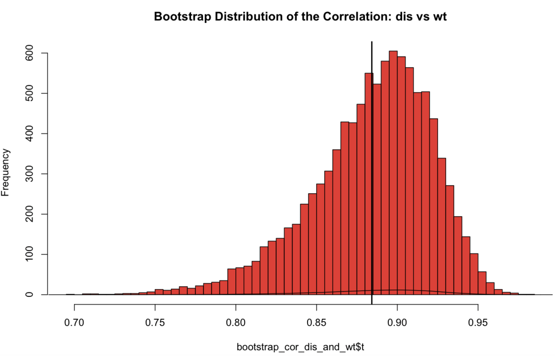
The results are as follows: t0 are the values of the statistic (i.e., correlation) in original dataset,
t is a matrix of 10000 rows (i.e., number of bootstrap repetitions) that we use to draw our estimate of this correlation.
The original mean value is 0.8879799 and the bootstrap estimate of the mean is
very close at 0.8842047, with a 95% CI between 0.8183 and 0.9652. Therefore,
disp and wt are strongly and positively correlated.